Overview

The goal of this assignment is to recify images and combine several images into a single mosaic. Rectifying images involve finding the homographic transformation between the image and a predefined geometry. Combining images requires both alignment and cross-dissolve. For alignment, we need to find the homography between the points in the source image and destination image, before blending them together.

Shoot and digitize pictures

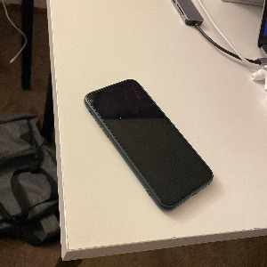
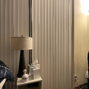
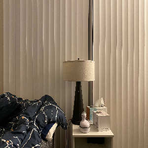
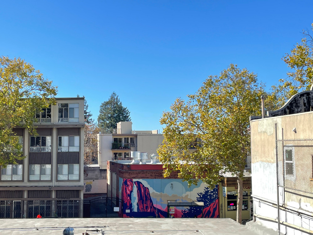
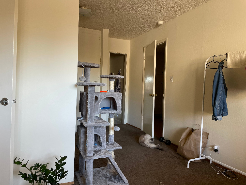
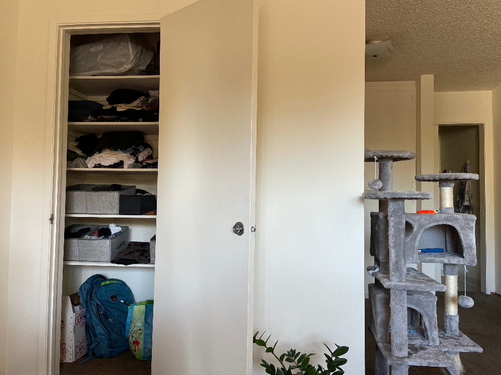
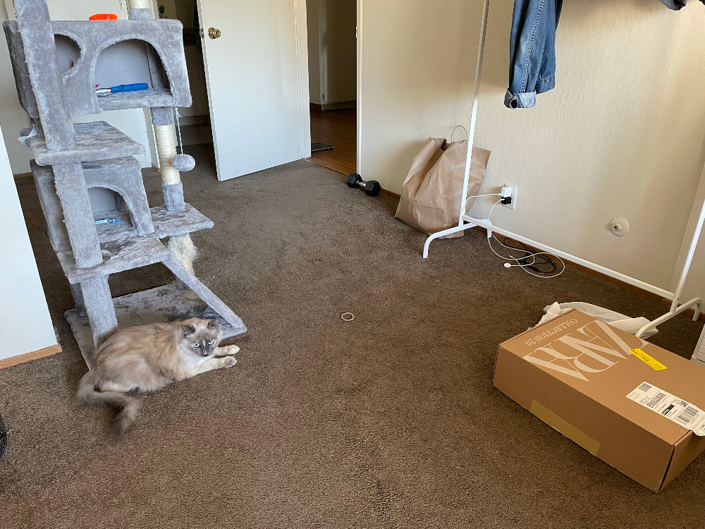
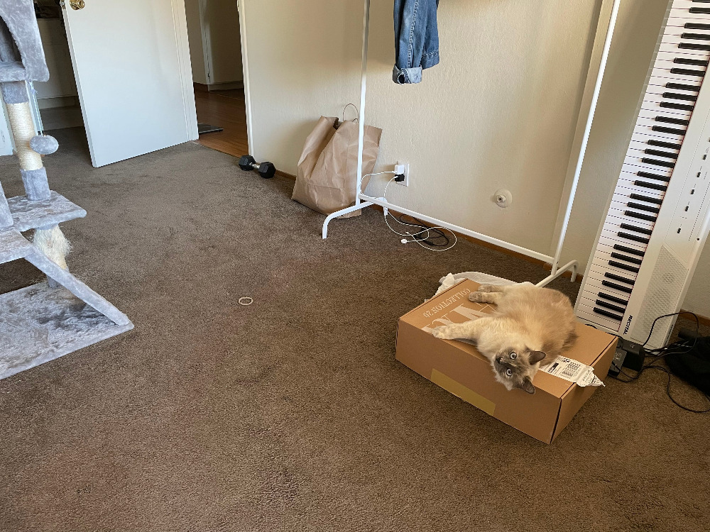
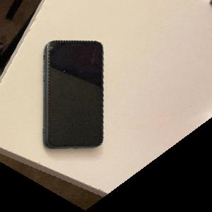
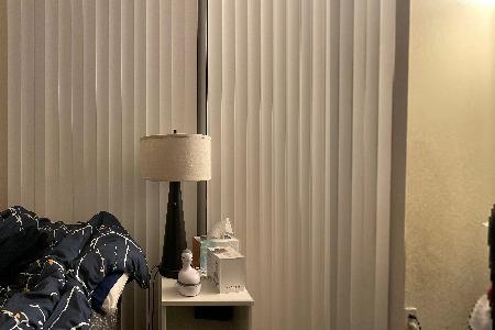
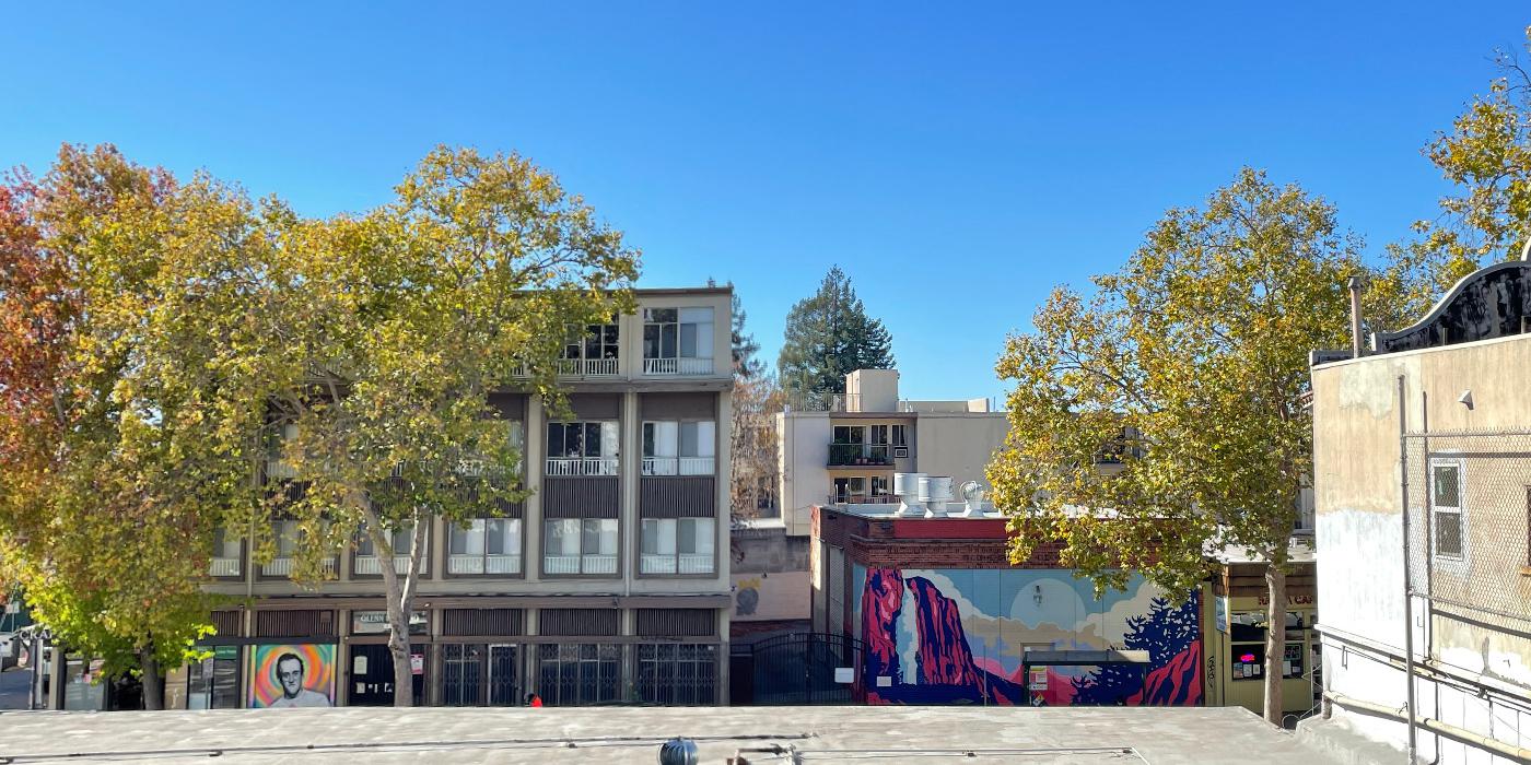
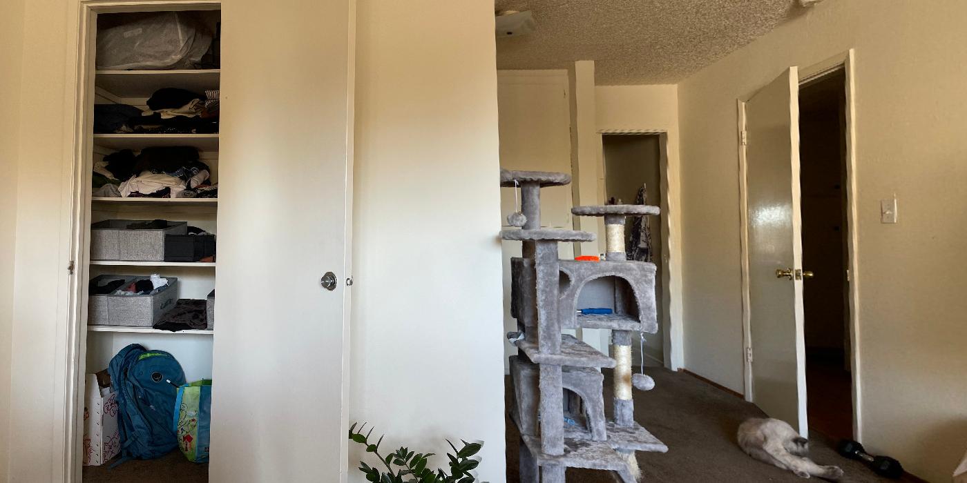
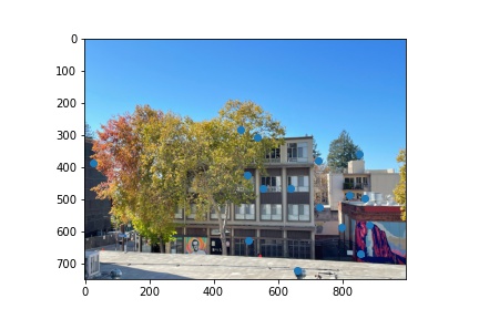
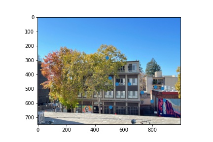
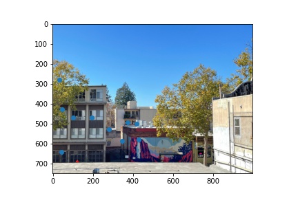
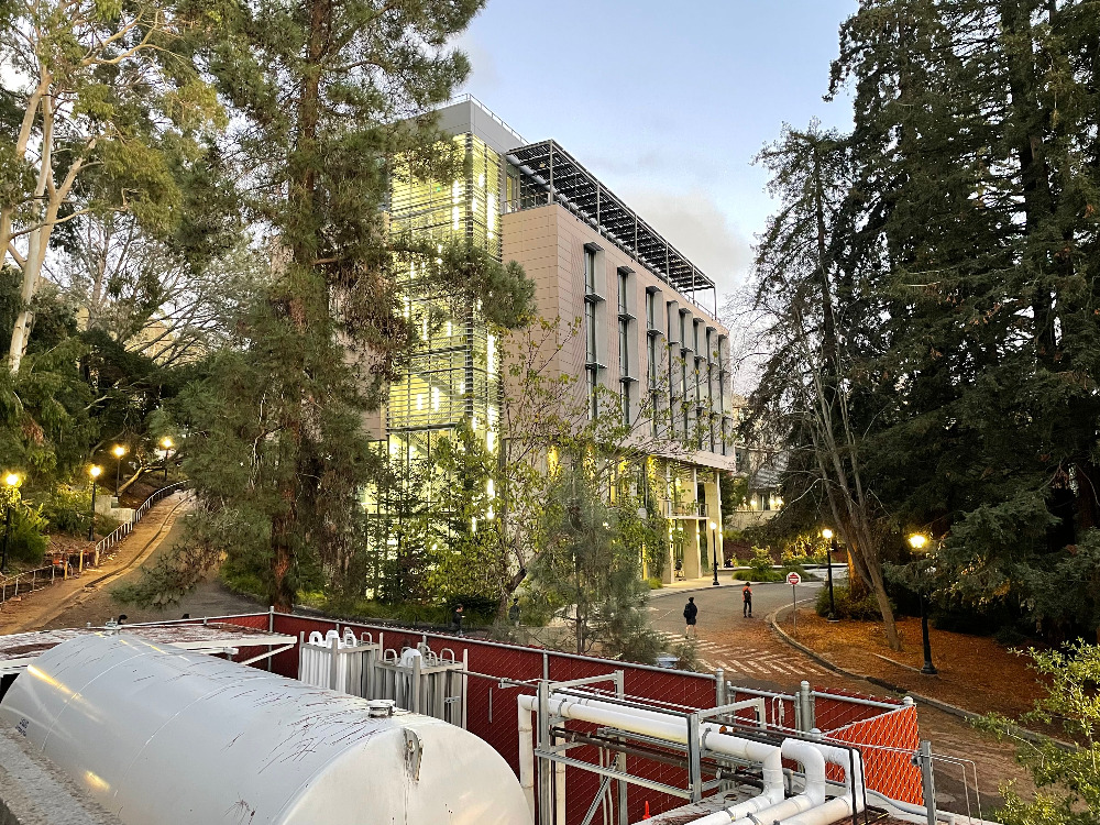
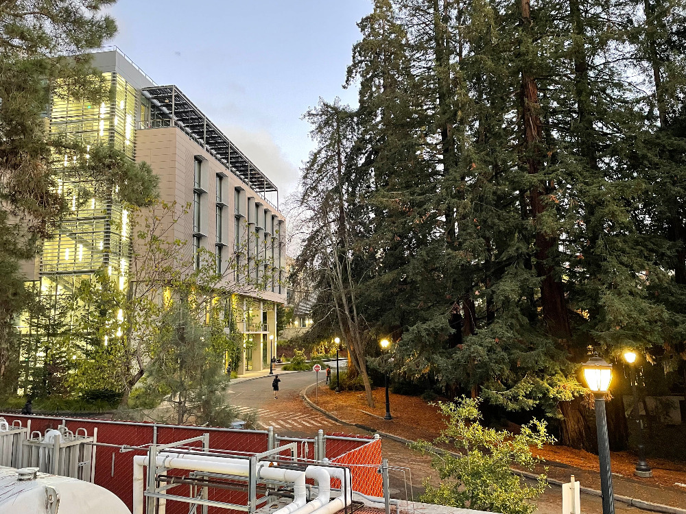
First, we need to have images to work on. I took photos of both indoors and outdoors, from the same point of view but with different view directions. I also made sure there are overlapping fields of view so that we can establish correspondence between images.

The below images shows the photos I took:

Recover Homographies

In order to do alignment between images or rectification, we need to recover the Homographies. The first step is to establish correspondence between corresponding points in source and destination images.

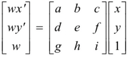
The homography matrix H is a 3x3 matrix connecting each pair of corresponding points. As shown in the formula below:

To solve matrix H, we need to vectorize this system of equations and include more data points. As seen above, it has eight degree of freedom, which means at least 4 points' corrdinates are required. Howvever, to reduce noise, we often select more correspondance than 4 to make the system overdetermined. Thus, the matrix H can be approximated using least square.

The vectorized equation is:

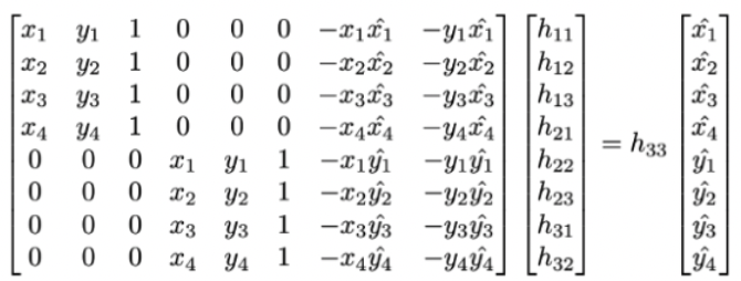
Warp the Images

After defining the correspondance, we can recover the homographies with the equation above. I used inverse warpping to avoid holes in the resulting image.

I first use the recovered homography to identify the size of the warpped image by warpping four corners of the original image. Then I used inverse warpping to find the coordinates in the original image and then interpolate these pixels. Lastly, we just put the interpolated values back to the resulting image. It's important to note that we need to scale the resulting coordinates by the third value (w) after warpping with homographies.

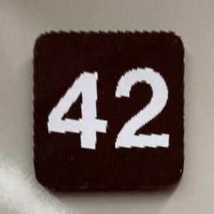
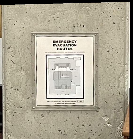
Image Rectification

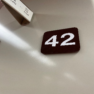
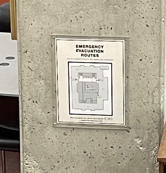
Image rectification is a good way to test our warpping method. In this task, I warpped some photos to make the object in the photo frontal-parallel. In all the following images, I first picked some planar points (usually the corners of the object). Then I define some corresponding points based on my knowledge of the object's frontal-parallel aspect ratio. I used my method above to recover the homography, and then use the recovered homography to rectify the entrie photo to be frontal-parallel.

Below are some examples of the origianl images and the rectified face.

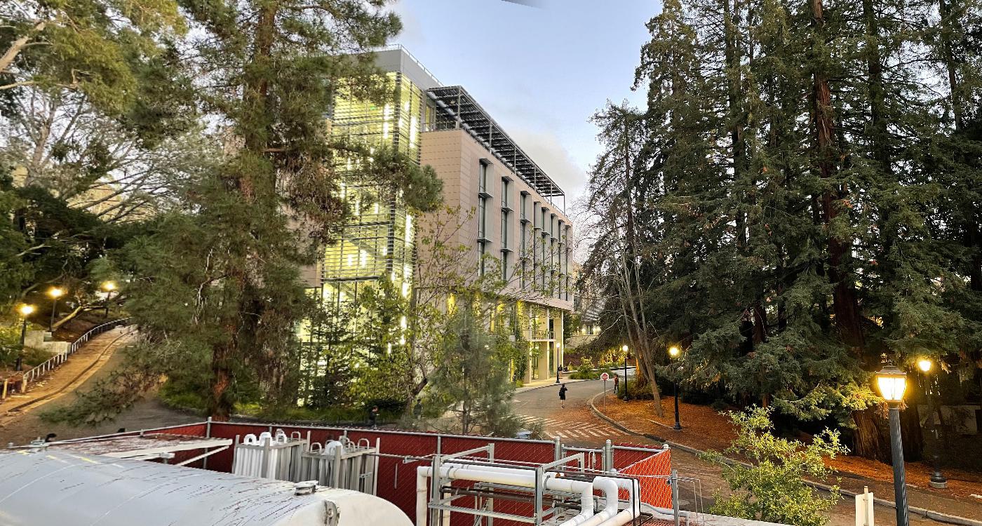
Blend the images into a mosaic

Now we are ready to blend some images!

To blend two images, we need to identify correspondance between the imageas. Then We can recover the homography. I used inverse warpping to ensure consistent result. With the homography, I first warpped the corners to find out the shape of the resulting image. Then for all pixels in the warpped image, I found the coordinates of their counterparts in the source image. I used these coordinates for interpolation. Lastly, I put the interpolated value back to the warpped image. This will make the two image aligned.

With the aligned images, we need to blend the colors together. We can not simply overlap them, because this will have edge effects. I implemented a two level Laplacian Pyramid to ensure smooth blending.

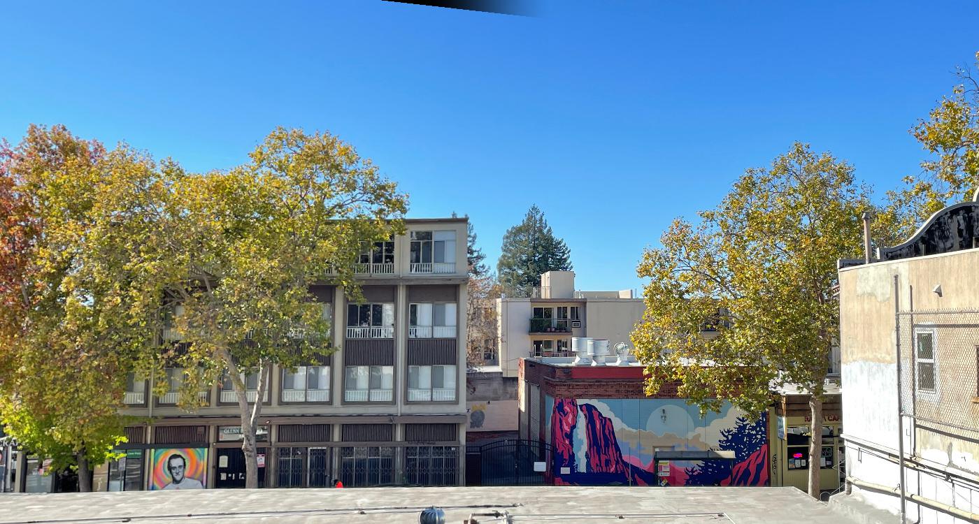
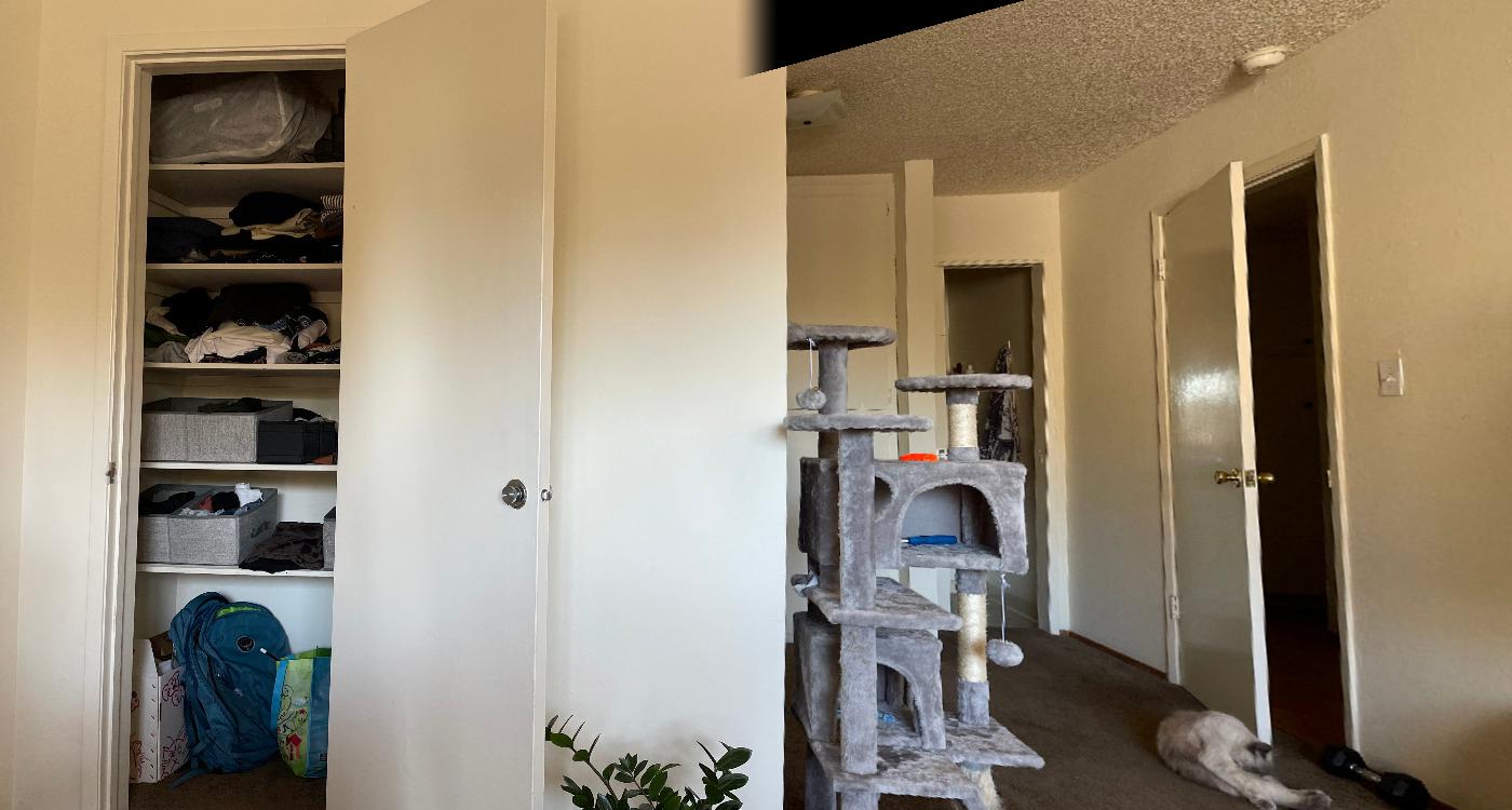
Below are some exmaple mosaics I blended:

For blending together more than two images, we can blend them one by one, using previous output as the input for the next blend, slowly growing the mosaic.

Part B: FEATURE MATCHING for AUTOSTITCHING

Step 1: Detecting corner features in an image

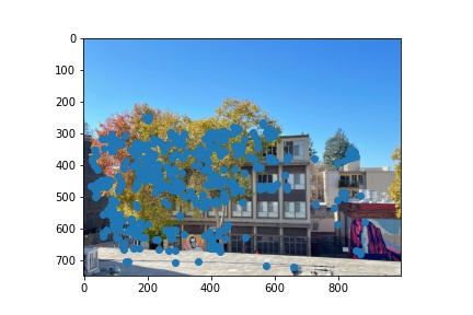
To achieve feature auto-detection, first we find all the harris corner in the image. We also compute the corner strength function of each pixel.

Since the computational cost of matching is superlinear in the number of interest points(corners), it is desirable to restrict the maximum number of corners extracted from each image. We also set a threshold to filter out corners that are too weak (below the threashold). Natually, we want to use the corners with the strongest corner strength to match features. However, we also want the corners to be spatially well distributed over the image, since for image stitching applications, the area of overlap between a pair of images may be small. To satisfy the requirements, we used adaptive non-maximal suppression (ANMS) to select a fixed number of interest points from each image.

As we can see, ANMS achieves better spatially distributed corners than naively selecting the strongest.

Step 2: Extracting a Feature Descriptor for each feature point

Once we have determined where to place our interest points, we need to extract a description of the local image structure that will support reliable and efficient matching of features across images.

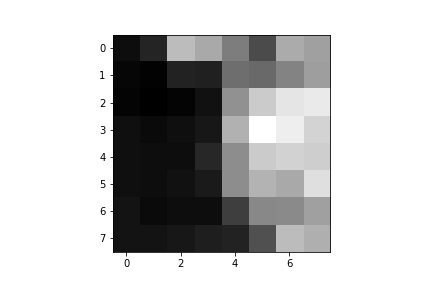
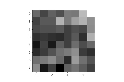
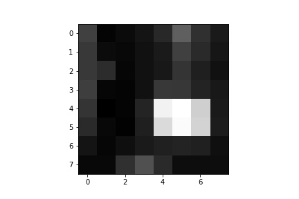
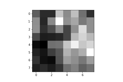
We find such descriptor of each interest point (corner) by sampling the pixels at a lower frequency than the one at which the interest points are located. Specifically, we find the 40x40 patch with each interest point as the center, then downsample the patch to be 8x8. After sampling, the descriptor vector is normalized so that the mean is 0 and standard deviation is 1. This makes the features invariant to affine changes in intensity(bias and gain).

We perform the above operation on each interest point to get an array of feature descriptors. Here are some examples of them:

Step 3: Matching these feature descriptors between two images

After generating an array of feature descriptor for each image, we need to match them. The basic idea is that we want to find patches that are most similar(1-NN) to each other. Specifically, we can do this by calculating the SSD for each patch with all other patches in other images. Then we choose one feature descriptor in each image that is closest to it. In this way, we can form a set with one patch per image for each patch.

Here we leverage Lowe's technique to also find the second most similar match for each patch (2-NN). We threshold on the ratio of (dist(1-NN) / dist(2-NN)) to selected the matches. As in Lowe’s work, we have also found that the distributions of dist(1−NN) / dist(e2−NN) for correct and incorrect matches are better separated than the distributions of dist(1−NN) alone

Here are the selected points after matching the feature descriptors:

As we can see above, there are still some features that are misclassified as corresponding pairs. We need to further filter out these outliers.

Step 4: Use a robust method (RANSAC) to compute a homography

To use the matched feature descriptor to construct a valid homography, we use Random Sample Consensus to further get rid of outliers, since least square is very unstable with outliers.

Specifically, we randomly select four feature descriptor pairs. We use these four pairs to compute homography H exactly. We then use the computed H to transfrom all descriptors in one image, and see how close they get to their counterparts in another image. We threshold this difference in distance to select a set of outliers.

We iterate this process for 1000 times and keep track of the largest set of inliers. Finally, we use this largest set to re-compute least square homography estimate on all of the inliers.

Here are the largest set of inliers selected by RANSAC algorithm:

As we can see now, the pairs of selected features after RANSAC are all correctly identified.

Step 5: Create a mosaic!

Finally, we combine all the steps above, with the blending steps from Part A, to create a mosaic. Below I compared the automatic feature detection results with the manual feature selection results.

We also use this algorithm on a new set of images:

As we can see, auto-stitching gives better results. An example is in the second panorama, the wall in the middle of the image seems to be parallel to the door frame on its left, which logically should be so. However, in the manual stitching panorama above, the wall and door frame do not look very parallel. This may be due to nosie introduced during manual points selection.

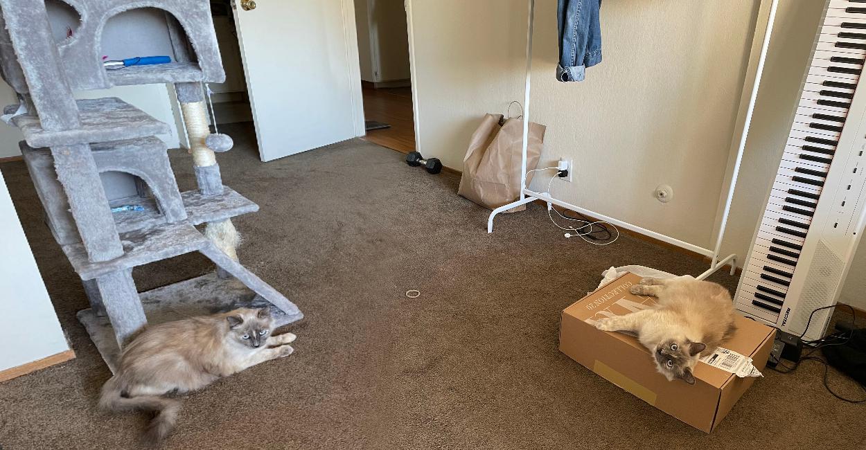
Bells and Whistles: Cat Replication!

Now I have two Nilas!

Final Thoughts

It is indeed very fun to work on this project. I used to use Photoshop to stitch photos together, but it was very high level. Now I really know the math behind this cool technique. One thing to note is that please remember to scale the warpped x and y by the third value of the warpped coordinates. Also, larger size and sigma gaussian kernel in Laplacian pyramid gives smoothier transition between images. However, the down side is that it takes really long to run!