Shoot and digitize pictures
Example 1
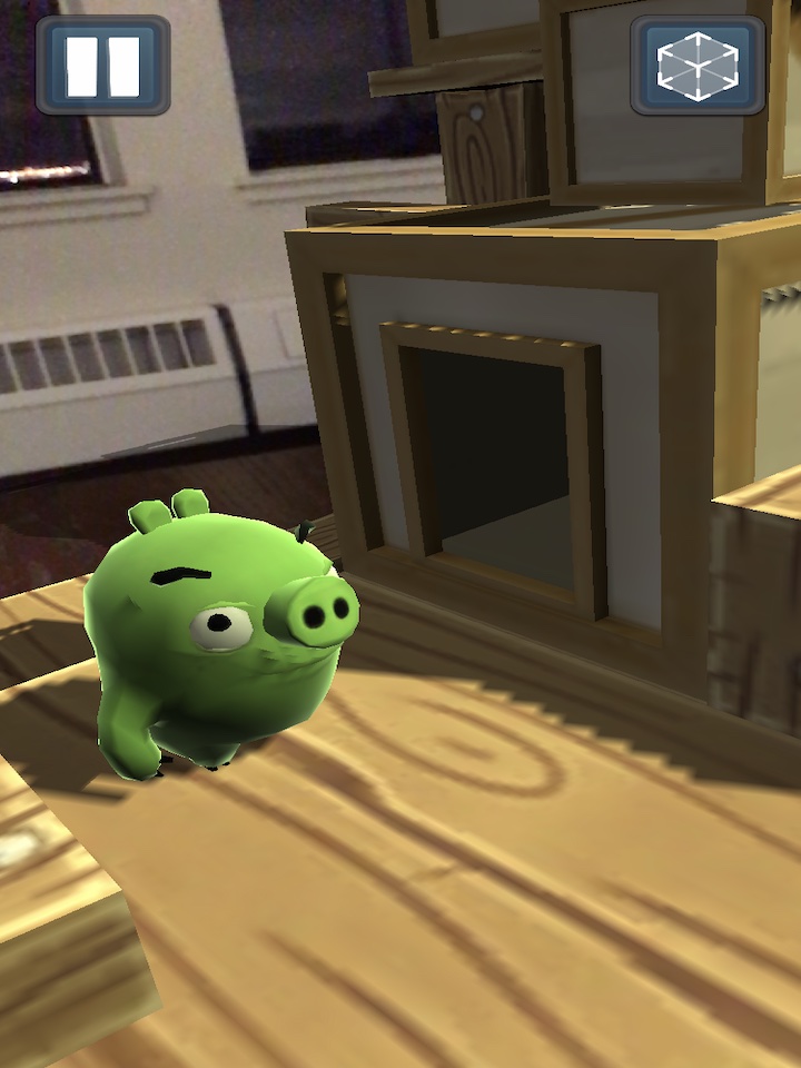
I used an iPhone with AE/AF lock when necessary, and resized images to 720x960. Some images are from my photo library and may have been taken with earlier phones, or as screenshots of e.g. Angry Birds AR Isle of Pigs.
Recover homographies
For this part, I coded a code to recover homographies. It would express the problem as a Least Squares. The key innovation is that though the matrix being recovered was 3x3, I rearranged the matrix into a 1x9 vector. This required flattening the output matrix into a vector, and creating individual rows for each subset of the input matrix that would multiply to the output matrix.
The end result is that you can solve for the homography matrix using A = one set of correspondences, x = the transform matrix, b = other set of correspondences. The interesting part is that just with this setup, the bottom row of the matrix will be nearly equal to 0, 0, 1 as expected, without any further constraining of the least squares, problem, because of how homogenous coordinates work.
Warp the images
Example 1
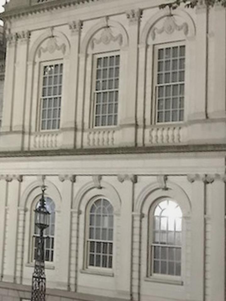
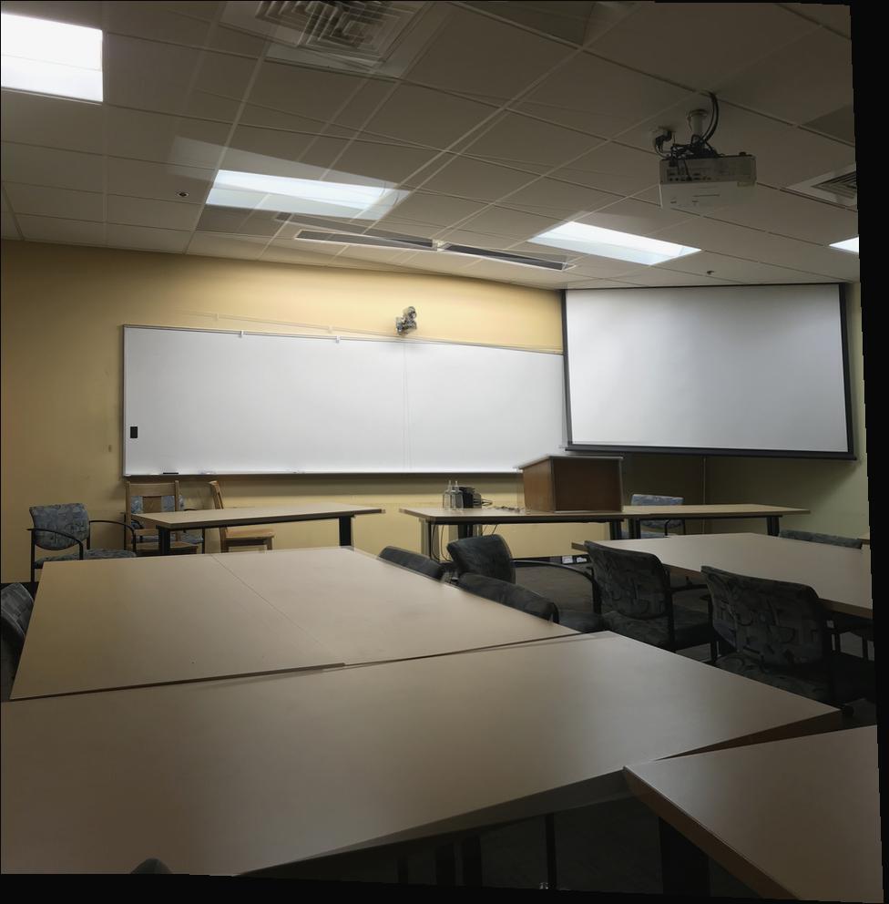
Original image:
Rectified wall of building.
Example 2
Original image:
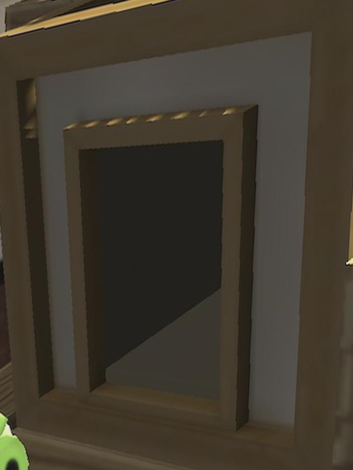
Rectified outer cube.
Blend images into mosaic
For this part, I estimated the size manually using a conservative estimate. That conservative estimate would guarantee that the full image is captured. I would then use magick mogrify -trim to trim out any blank space in all the output images.
One thing I noticed was that having low quality correspondences would reduce the quality of the final mosaic, which could cause difficulties.
For alpha feathering, I used a simple linear function of distance from the center to create a smooth blend. This would only apply when multiple images had pixels in the same location.
Example 1
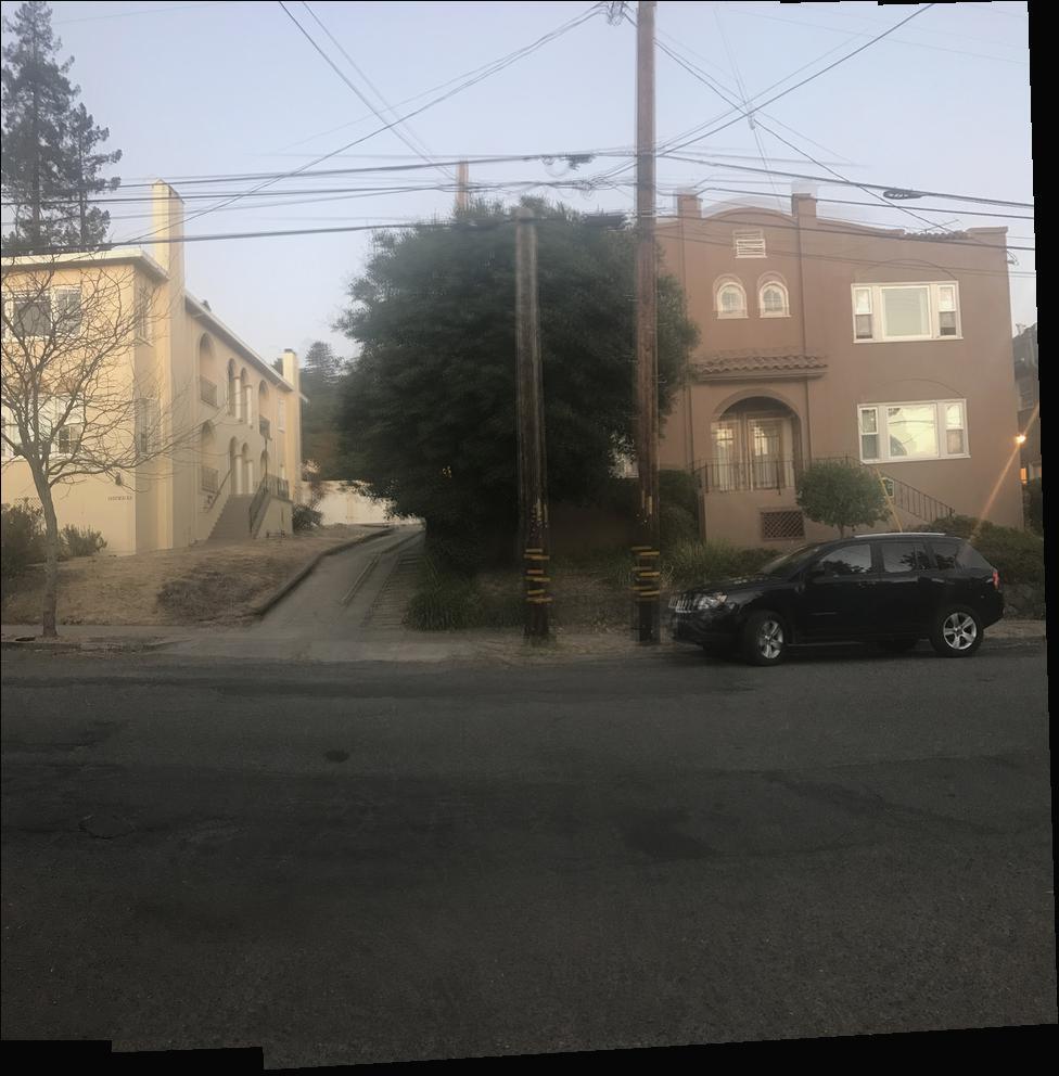
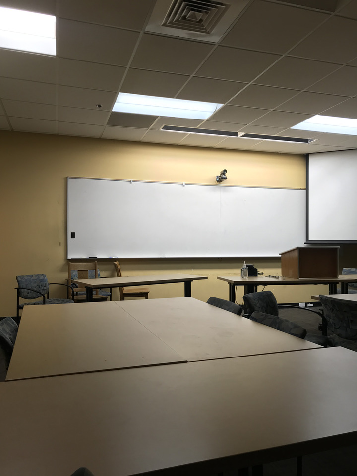
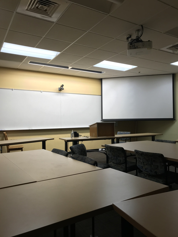
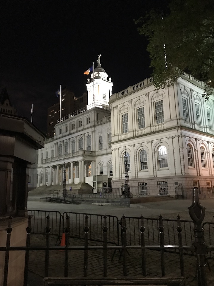
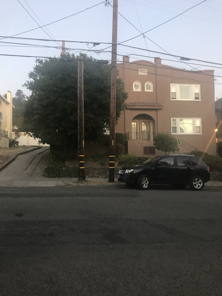
Original images:
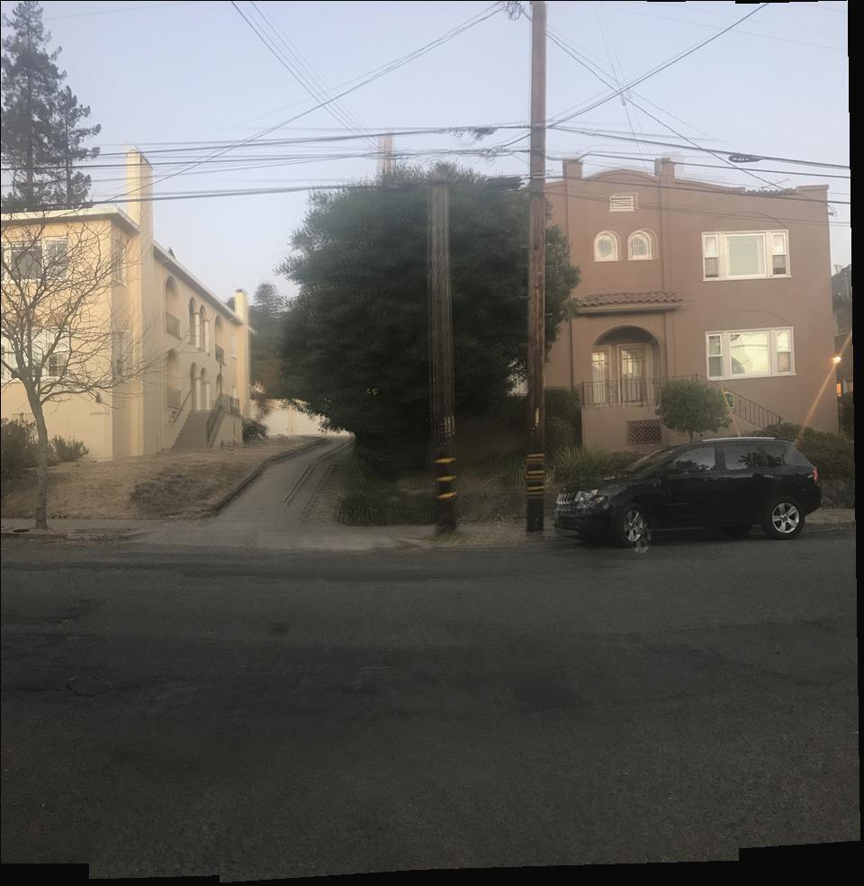
Mosaic image:
Example 2
Original images:
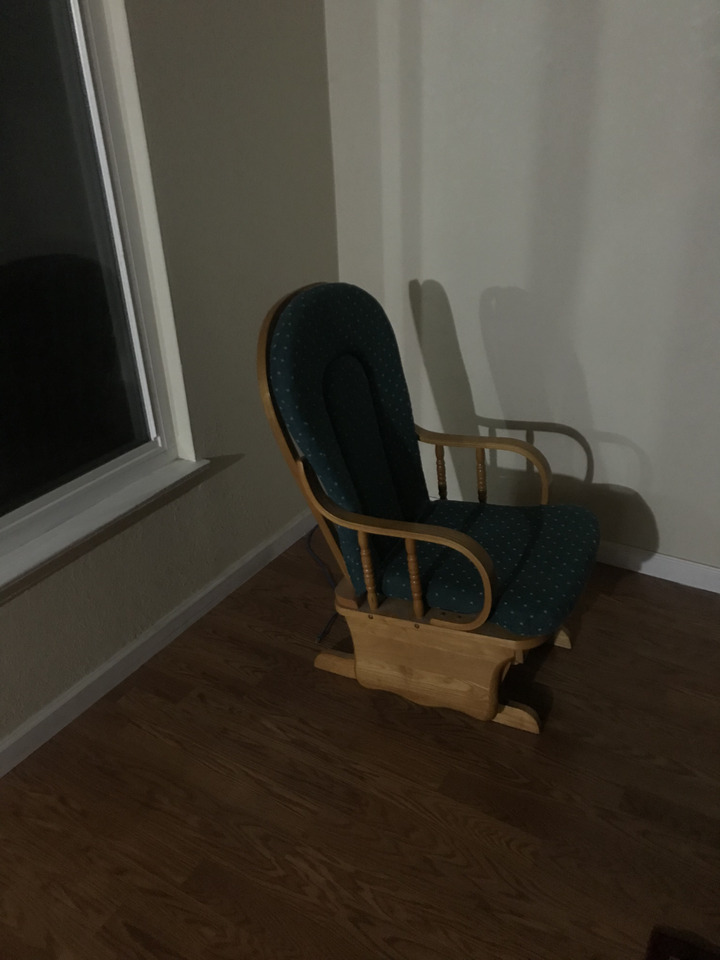
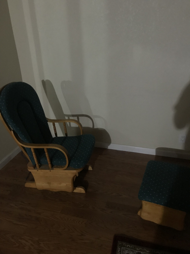
Mosaic image:

Example 3
Original images:
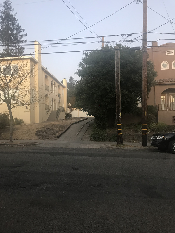
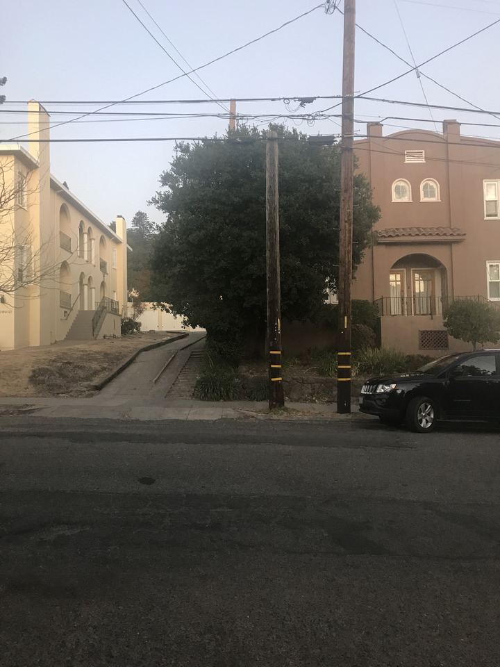
Mosaic image:
What you learned
What I learned from this project is the importance of smoothly interpolating masks, as otherwise the transform looks much worse at the edges. I also learned that not vectorizing code can severely negatively impact performance. Also, I learned that labeling a lot of correspondence points is not useful. It's more important to have two images that are good matches for each other so that the general transform can work in the first place, or its doomed.
When working on the the second part, I found and fixed a coordinate bug in my first part that had affected vertical coordintes. That allowed me to improve both my manual and automatic stitching as well as my rectification.
PART TWO: AUTOSTITCH
1. Detecting corner features in an image -- Harris corners on an image
For this part, I used the existing Harris sample code. The result can be seen on an image:
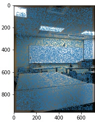
Adaptive NMS and Corners Overlaid on image
Next, I implemented Adaptive NMS to keep only Harris corners that were farthest away from similarly valuable corners. This was optimized with some vectorization to keep the runtime around a minute on 720x960 images. We can see the results with 10, 50, and 100 best corners kept:
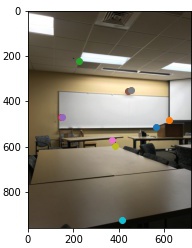
As we can see, the priority is first on getting good corner like features, but later it starts getting various spaced out points that are okay corners.
2. Extracting a feature descriptor
Extracting the feature descriptor is pretty easy, we can just sample from a 40x40 region of a blurred image (I used a Gaussian blur with sigma=5) with stride 5 to get the sampled feature for each part of the image. The blur is what makes the strided sampling still good.
3. Matching feature descriptors
Matching feature descriptors is also very easy, we can just go through and choose features that had a high maximum match relative to the second best match for another feature (I used a threshold of 0.7 based on the graph). Basically we're looking at the best match score (SSIM wise) / second best match score (SSIM wise) and higher is worse, so we want a ratio less than 0.7 for us to consider the match good and use it.
4. RANSAC homography
For RANSAC, I would choose random 4 points, and then compute homography and find the number of points that were within error 10 after reprojecting. The homography with the most matching points (inliers) was the final one used. What was cool was that since I was using a smaller number of features after NMS (200) I could get away with fewer RANSAC iterations (2500).
Auto-Mosaics compared to Manual Mosaics
Example 1
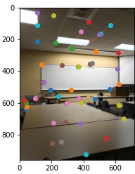
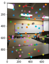
Original images:
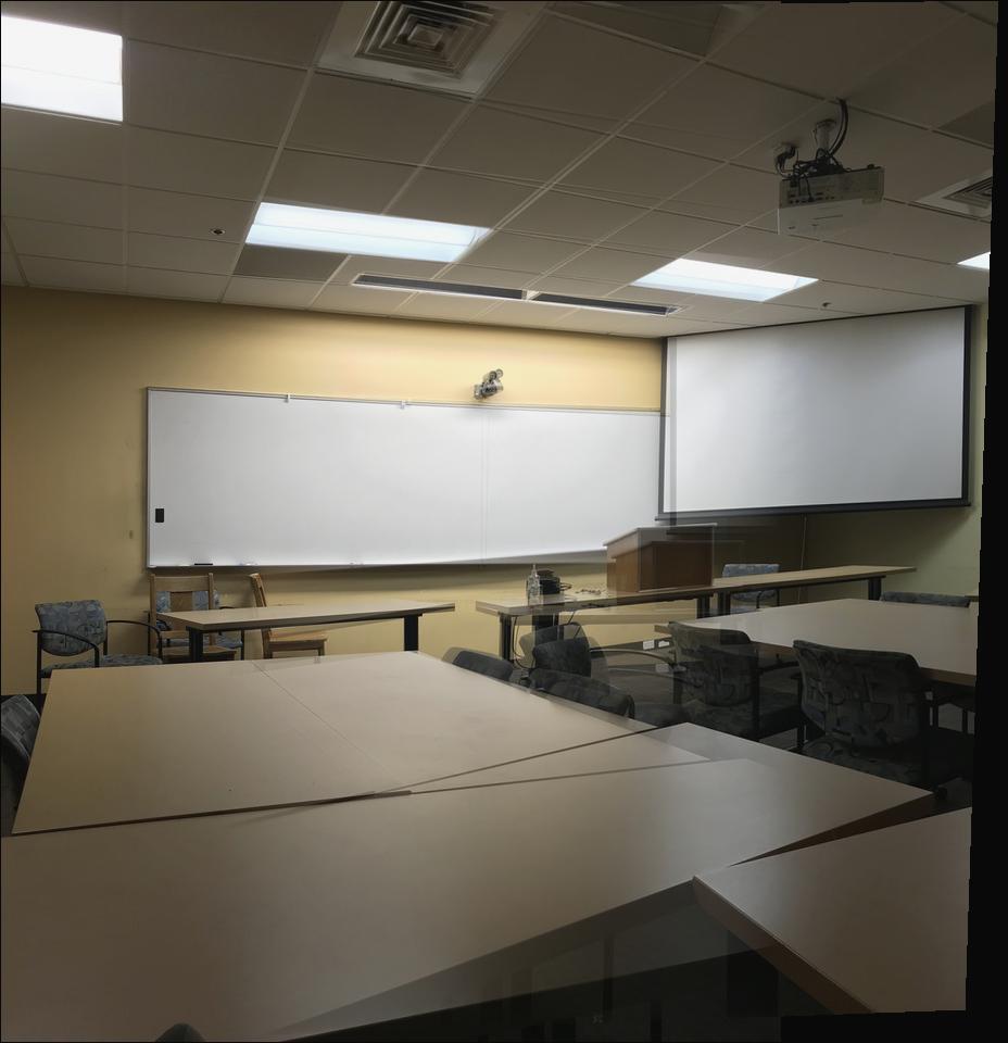
Manual Mosaic image (left) and Auto (right)
Example 2
Original images:
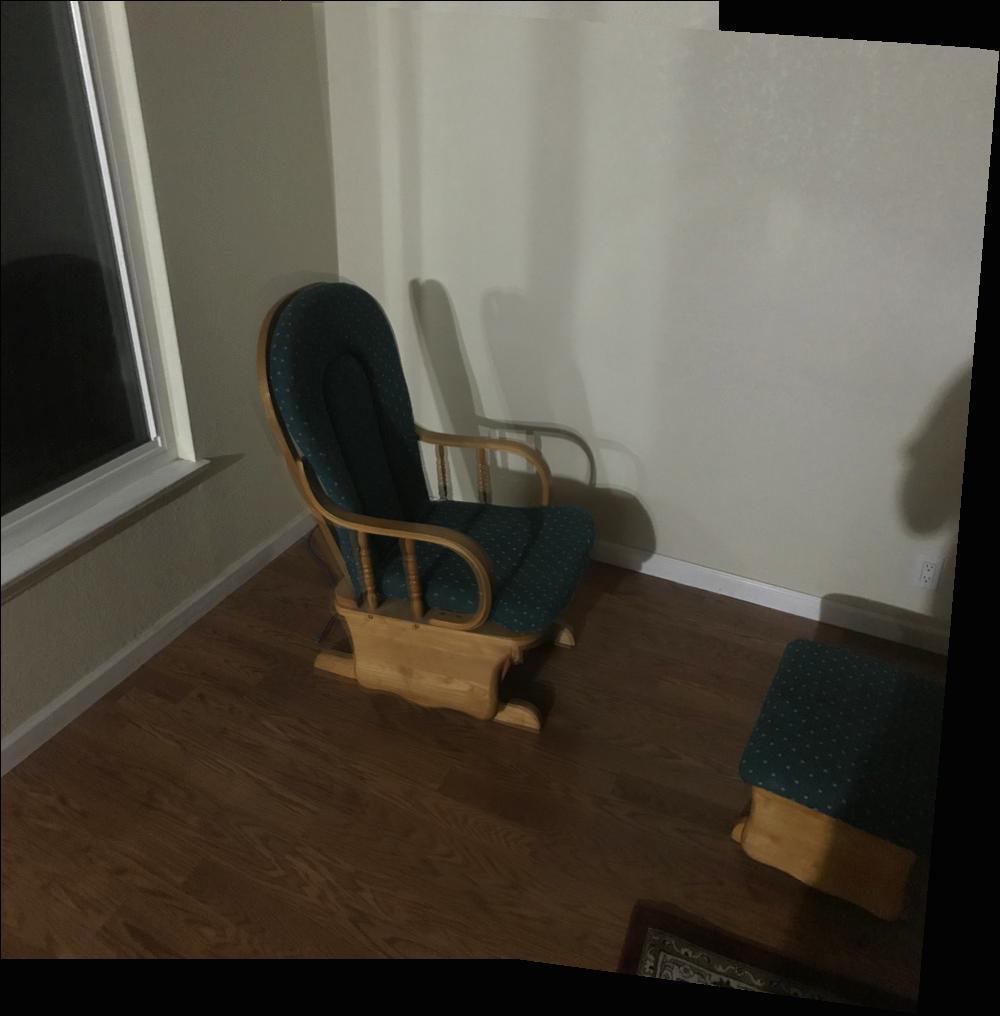
Manual Mosaic image (left) and Auto (right):
Example 3
Original images:
Mosaic image Manual (left) and Auto (right):