Project 4a

Homographies

I recovered homographies by using least squares, with the algorithm shown in the lecture slides.

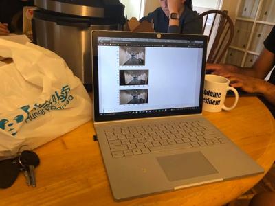
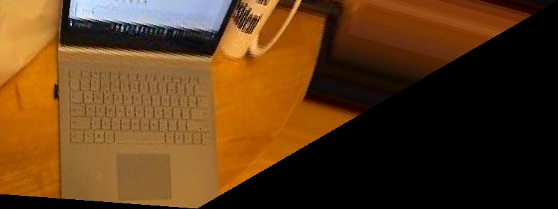
Rectify

To rectify, I selected the four points for the morphed rectangle in the image, and used the same morphing algorithm to morph the image to a manually coded rectangle in the middle of the image.

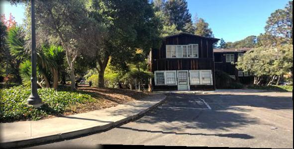
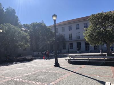
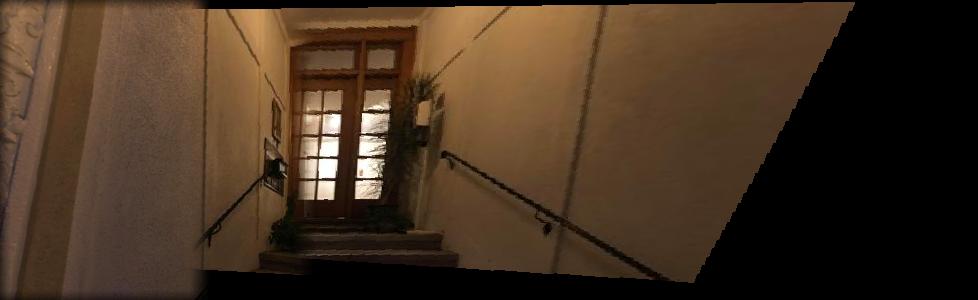
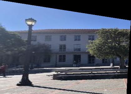
Unmorphed laptop image	Morphed laptop	Unmorphed building	Rectified building

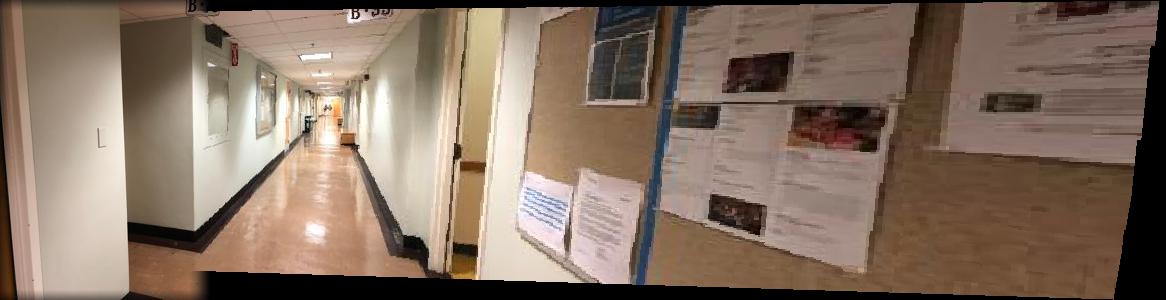
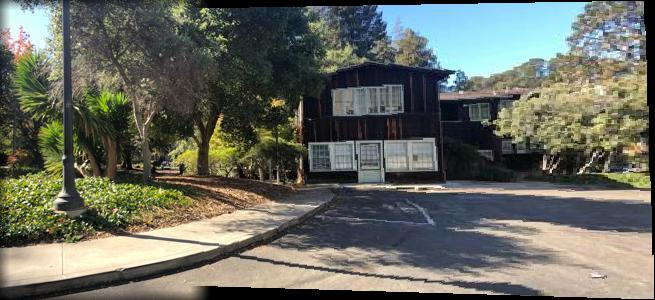
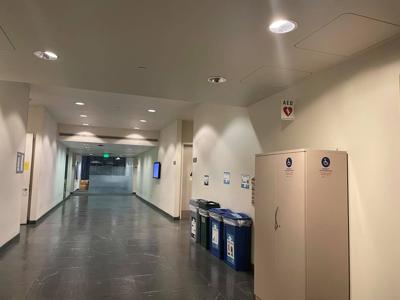
Mosaics

To stitch together mosaics, I created an array of images taken from the left-most pan to the right-most pan. Starting from the last image, I morphed the image to align with the previous image, then this combined image to match the image before it, etc. I stitched all of the images together using gaussian blending (the method in project 3, with a blurred mask).

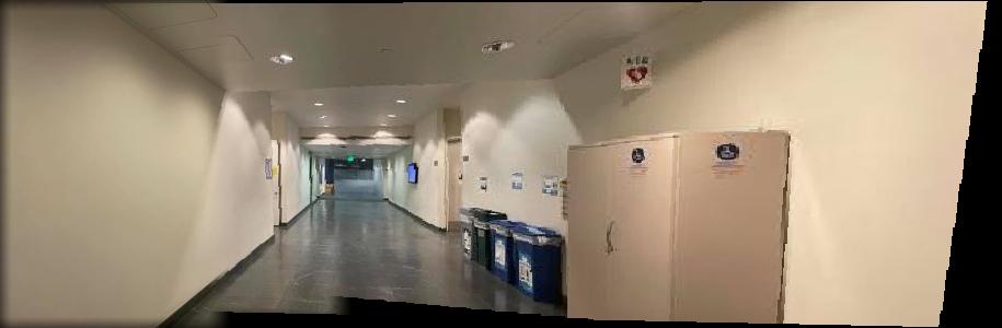
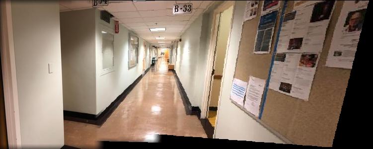
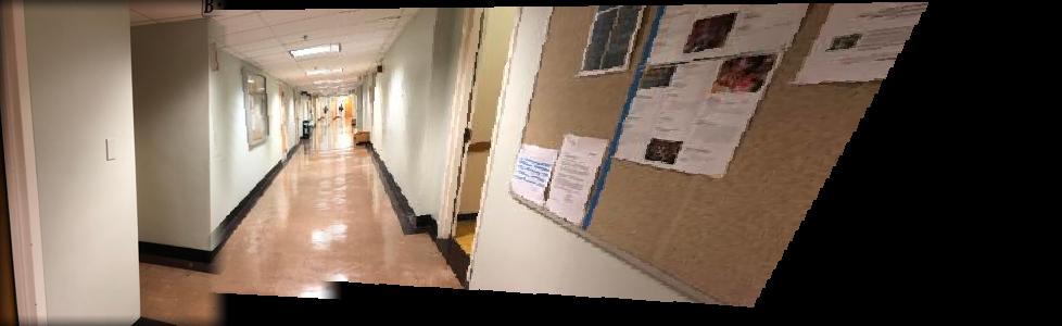
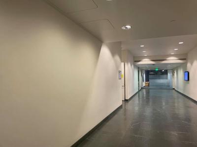
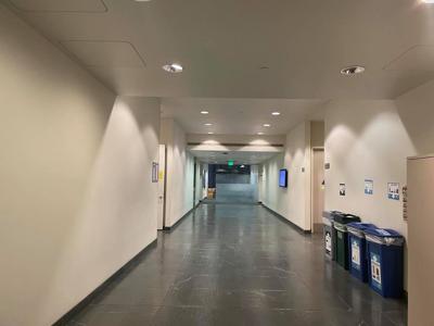
Panorama 1, img 1	Panorama 1, img 2	Panorama 1, img 3

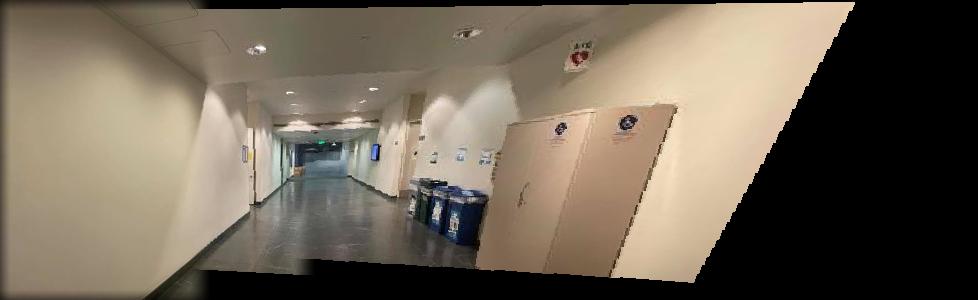
Stitched panorama 1

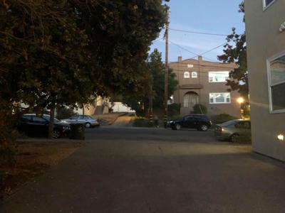
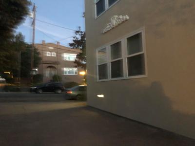
Panorama 2, img 1	Panorama 2, img 2	Panorama 2, img 3

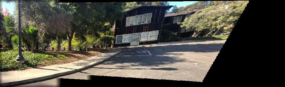
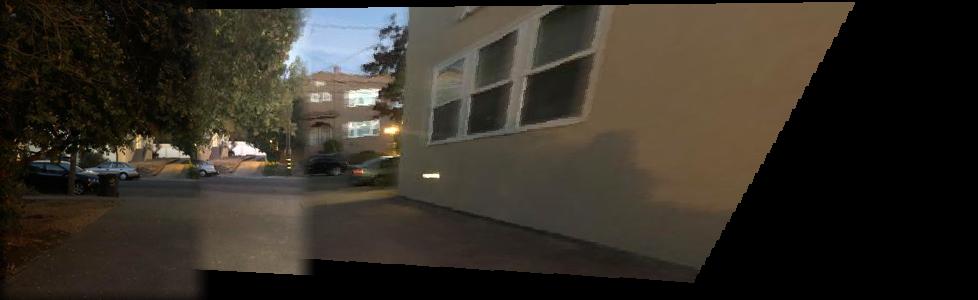
Stitched panorama 2

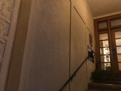
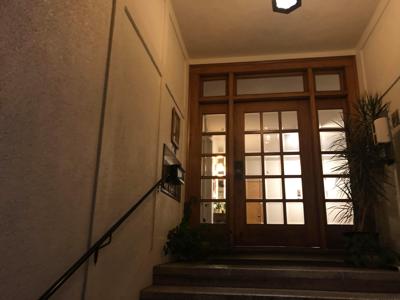
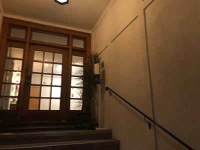
Panorama 3, img 1	Panorama 3, img 2	Panorama 3, img 3

Stitched panorama 3

Project 4b

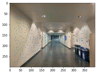
Harris points

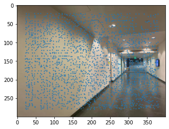
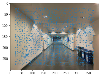
I used the built-in code to find a lot of harris points for each image in a given panorama.

Harris points for pano 2.1	Harris points for pano 2.2

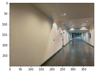
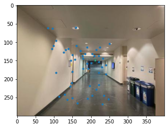
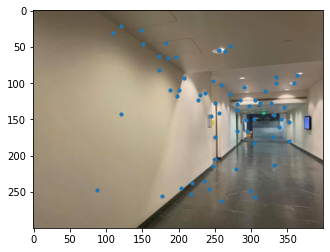
ANMS

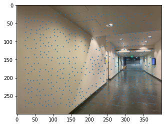
I implemented ANMS as described in the paper, using the top 500 points in terms of maximum non-suppressed radius. Here are the ANMS points on the above images:

ANMS points for pano 2.1	ANMS points for pano 2.2

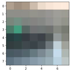
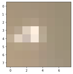
Feature matching

For feature matching, I created feature vectors for each point by downsampling a 40x40 image around each point into an 8x8 image as described in the paper, normalizing the image, then flattening the vector. For each point, I found the (different) point that had the most similar feature vector in terms of distance (using the provided dist2), as well as the second most similar point. If the ratio of the best distance to second-best distance was below the defined ratio (0.3-0.5, a hyperparameter), and if the best point was not already in a set of stored best matches, the match was added to the set of point matches. Here are the matched points for the above images.

feature example 1	feature example 2

matched points for pano 2.1	matched points for pano 2.2

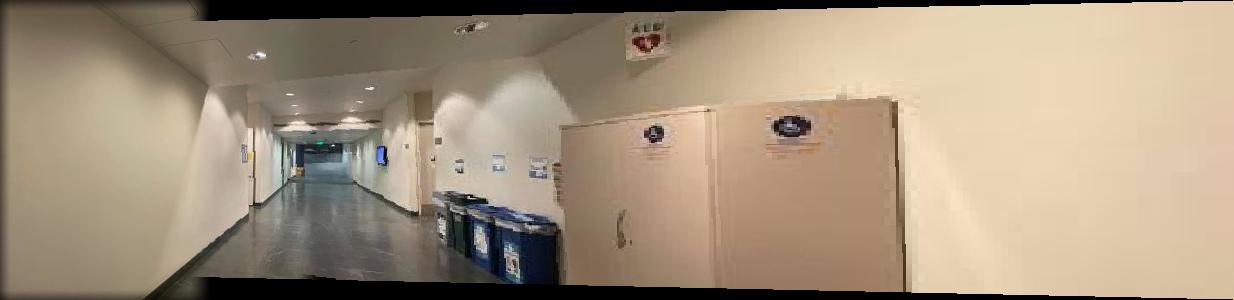
Below are the final auto-stitched panoramas on the left, alongside their manually-chosen-points counterparts on the right. In general, it seems like the auto-stitching worked better, likely as there were just more points and higher accuracy.

Auto-stitched pano 2	Manually chosen points pano 2

Auto-stitched pano 5	Manually chosen points pano 5

Auto-stitched pano 6	Manually chosen points pano 6

RANSAC

For RANSAC, I iterated 20k times, with a default point distance tolerance of 5 pixels, on the previously generated matched points.

Pre-ransac pano2.1	Pre-ransac pano2.2

ransac pano2.1	ransac pano2.2

Here are the above panoramas, stitched with the RANSAC-defined points, with the auto-stitched images for

Auto-stitched pano 2	RANSAC pano 2

Auto-stitched pano 5	RANSc pano 5

Auto-stitched pano 6	RANSAC pano 6

Using the RANSAC points gave some clear improvements in the panoramas: for example, in the first one, we can see that the square in the top left of the ceiling is broken in the auto stitching (and if you scroll up, the manual points), but the RANSAC chosen inlier points fix this.

Takeaways

Many of the algorithms, while initially daunting to read in the paper, were much simpler and worked much better than I expected. I suppose the main takeaway of this is that simple and smart solutions can often work very well, as we can see in the case of auto-stitching performing better than manual point selection.