Project 4A: Abel Yagubyan
Shooting the Pictures
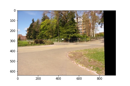
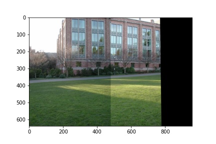
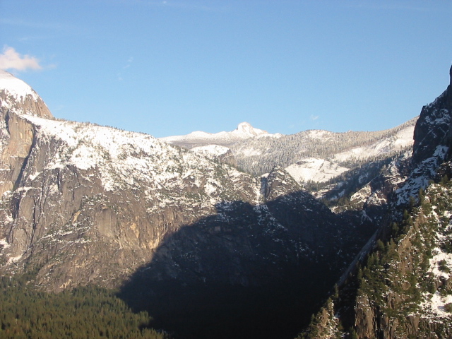
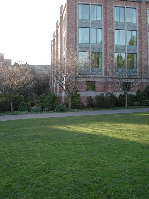
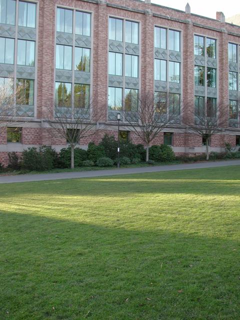
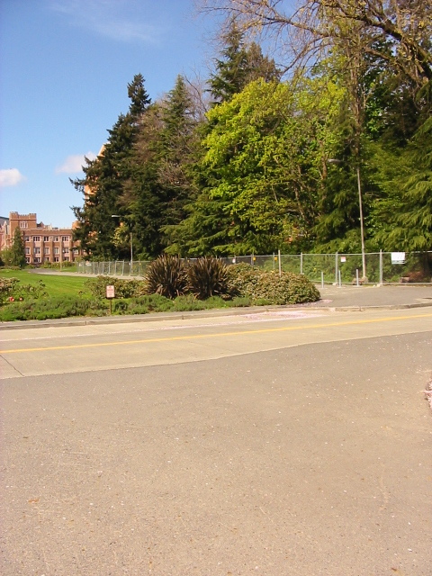
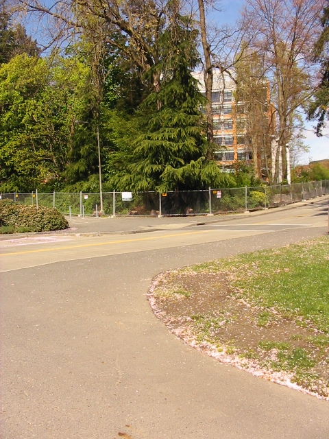
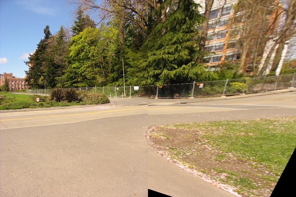
I attempted to take helpful images using my phone, however, the results were very suboptimal and not the greatest looking ones. Hence, I went ahead and used demo images from the dataset found in the following link. Here are some images below (image on the left is the left side, image on the right is the right side).
Recover homographies
I essentially recovered the homographies using the least squares method between the images, where I set up 4 and more correspondences between the images to use. By using these n amount of correspondences between the images, we were able to retrieve the H column vector (hence, 3x3 matrix) by solving the following equation below (also by allowing h_33 to be equal to 1). The equation was taken from the following link.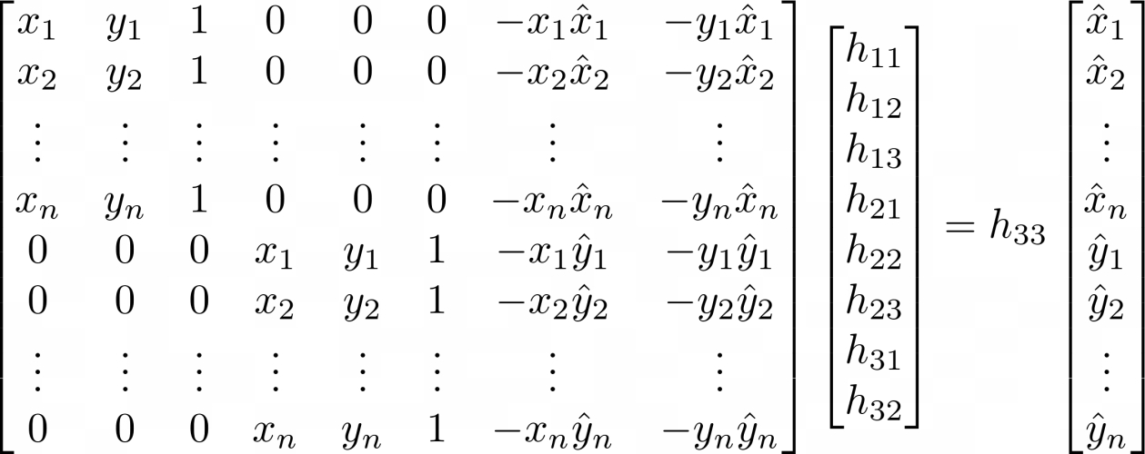
For instance, the H matrix for the first set of images above was equal to:
matrix([[ 1.18320210e+00, -1.36211424e-01, -3.66973729e+02], [ 1.15603031e-01, 9.22285758e-01, -5.38680254e+00], [ 4.89096096e-04, -5.48078324e-04, 1.00000000e+00]])
Warp the images
I wrote the warping function that essentially takes both of the images and the homography matrix as inputs, which then was applied to inverse warp to transform the second image into the base first image (by using cv2.remap), which were then placed next to each other and blended together as a final result.Image Rectification
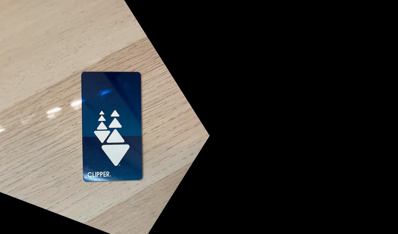
For testing purposes, I attempted to apply the rectifying technique on some images by warping some of the 4-sided objects to a "target straigtened" correspondence of the same object, which essentially straightens the object. Here are some examples (left side is original, right side is rectified version).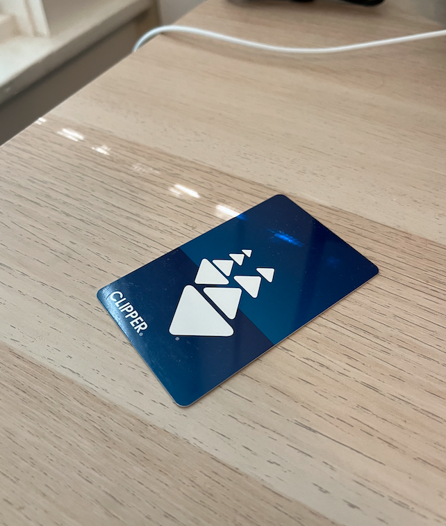
Blend images into a mosaic
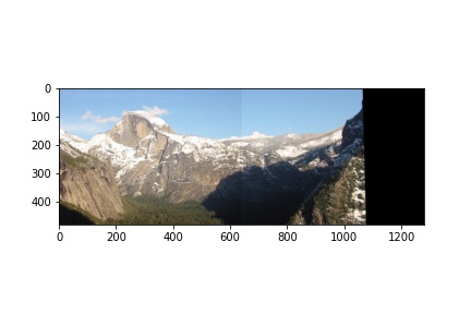
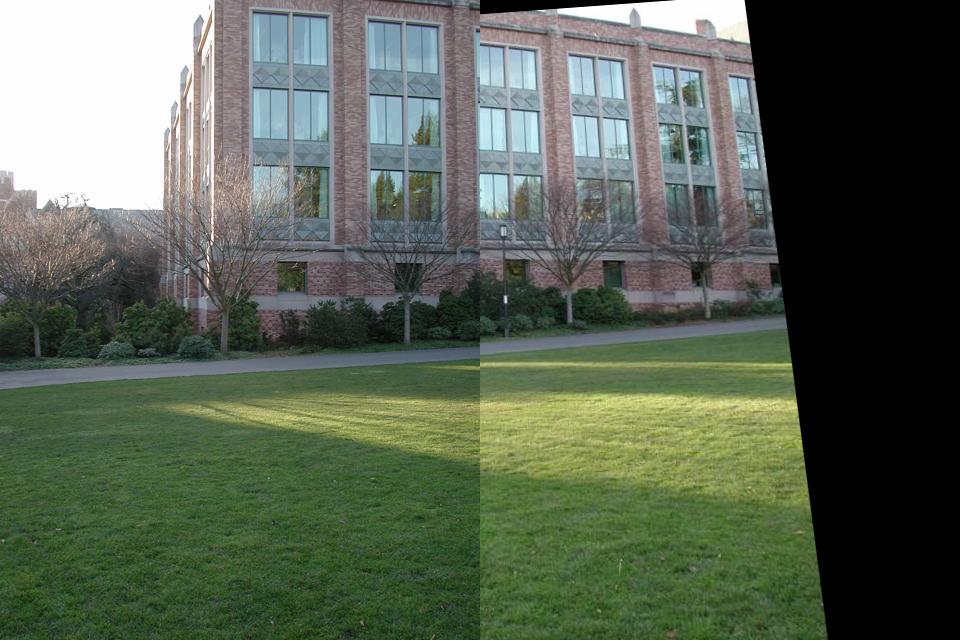
For the blending purposes of the mosaic, I used the warping function to smoothly combine the images by mapping the second image to the first, which was then blended together as a final output. As visible in the last 2 results, the images were not perfectly aligned due to the definition of the correspondences, however, the approach is still the same and produces pretty good mosaics as a result.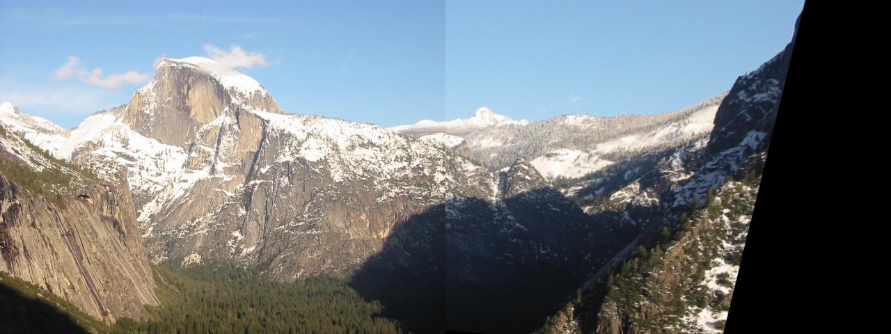
Project 4B
Harris Corners
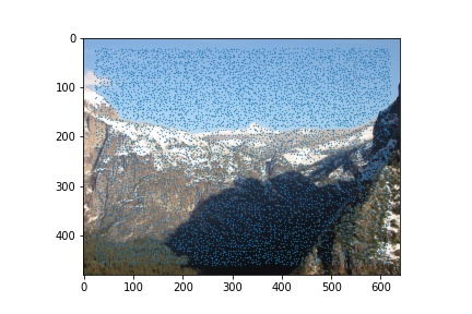
As mentioned within the lecture and the spec, Harris corners are used to identify features of images, hence we first run the code supplied in harris.py with an edge_discard value of 20. As seen below (left image is the left part of image, right image is the right part of image), there are way too many points. Hence, we might want to change our feature selection method.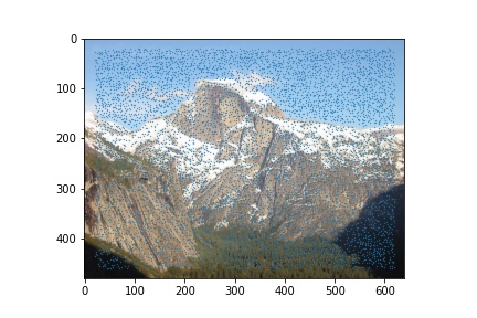
Adaptive Non-maximal Suppression
As mentioned above, we need a method to actually reduce and discard some of the features present within the image. To do this, we find the best possible corner around a point (using a radius and retrieving a radius of interest, where we begin with r = 0 and increment by 10 pixel for every iteration). I set the default amount of points to be reached to be 500 points (similar to the value in the paper), where we got much less and uniform amount of points (as displayed below).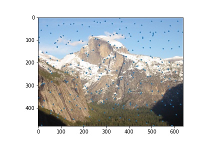

Extract feature descriptor for feature points
For every point attained from the ANMS method, we use a 40x40 Gaussian blurred pixel area around it and downgrade to a 8x8 patch, which is then normalized mathematically and set up as vectors to essentially become feature descriptors. Here is an example below: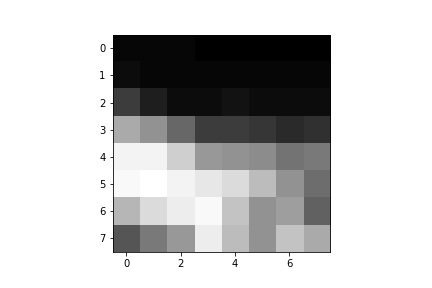
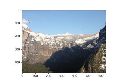
Match feature descriptors for two images
After having gotten the feature descriptors as mentioned above, we use SSD to compare the descriptors and use a threshold of 0.1 to essentially accept the best possible match for every feature. After having done so, we are left with the following features in both images: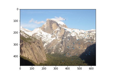
RANSAC and produce mosaic
Afterwards, we use the RANSAC algorithm taught in the class to compute the best possible homography matrix from all of the possible feature matches by randomly sampling 4 matches and then computing its homography matrix using the function implemented from part A. With this homography matrix, we apply it to the second image and check the amount of matching points present in the other image by keeping track of the inliers present. The best possible homography matrix is chosen and then used to produce a mosaic using the code from part A. Here are some cool examples of mosaics that worked out well (notice how drastically better they look than the manually picked ones from part A!):