In this project I rectified images and formed image mosaics by using homographies to align the images together.
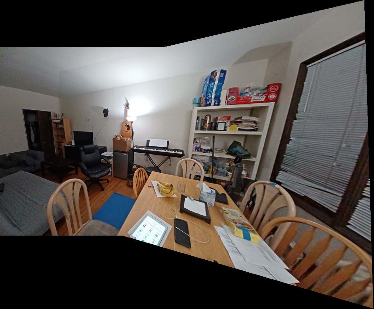
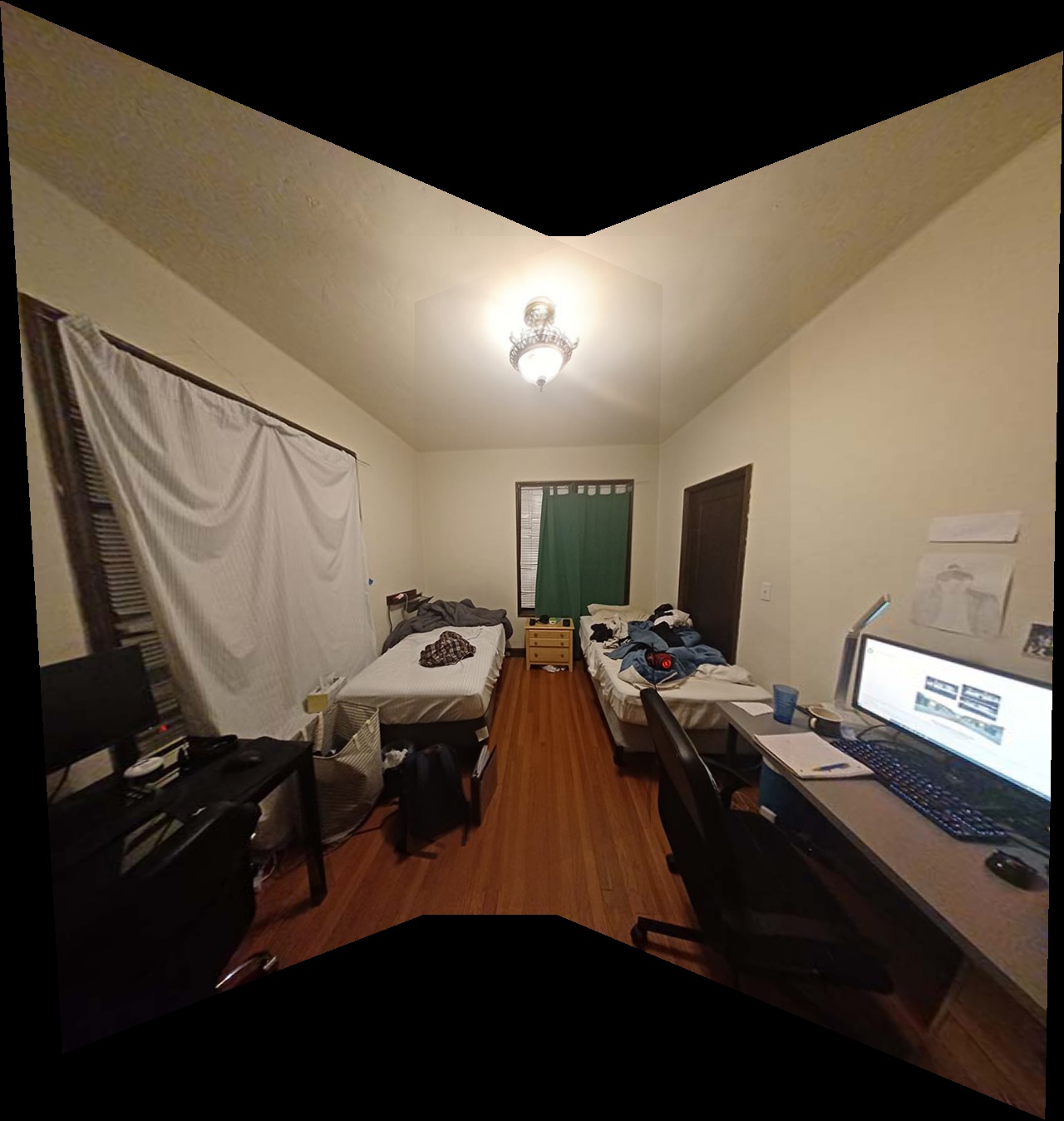
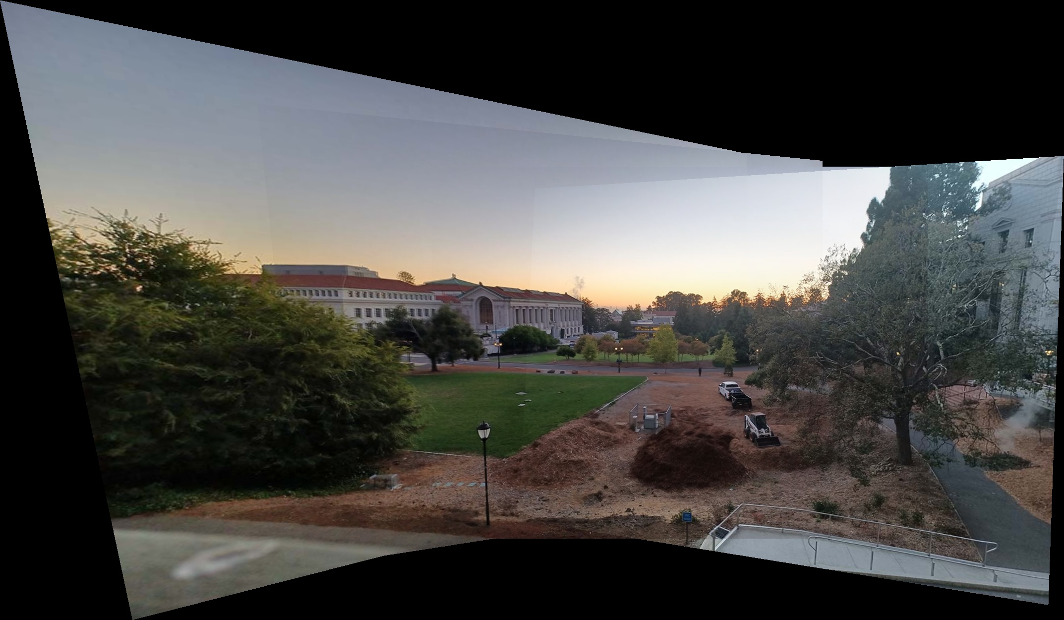
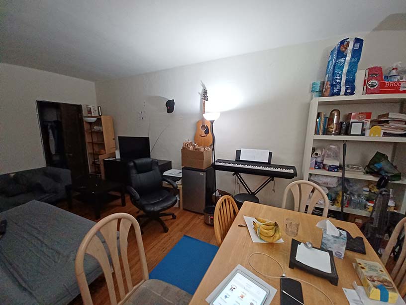
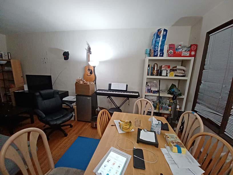
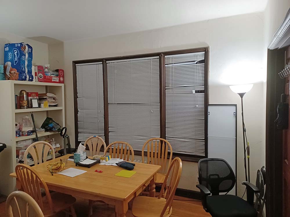
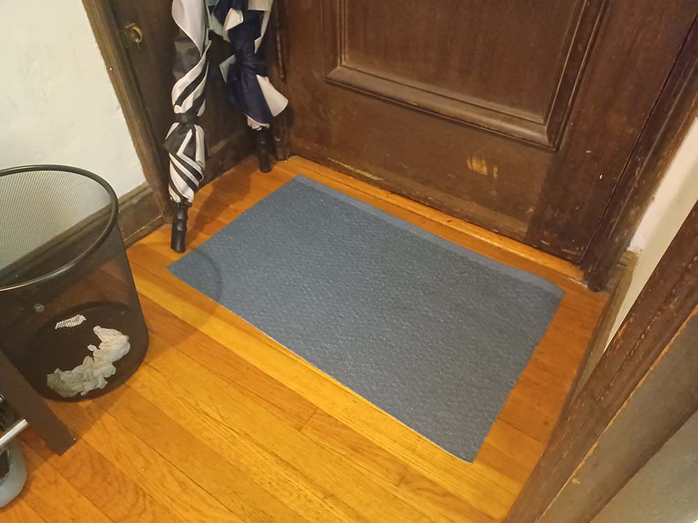
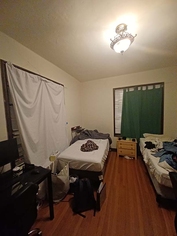
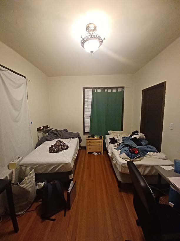
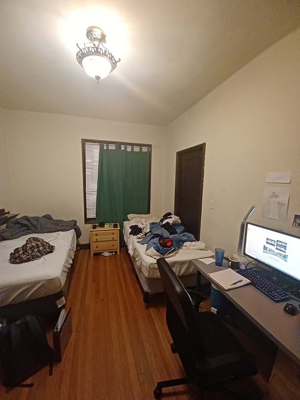
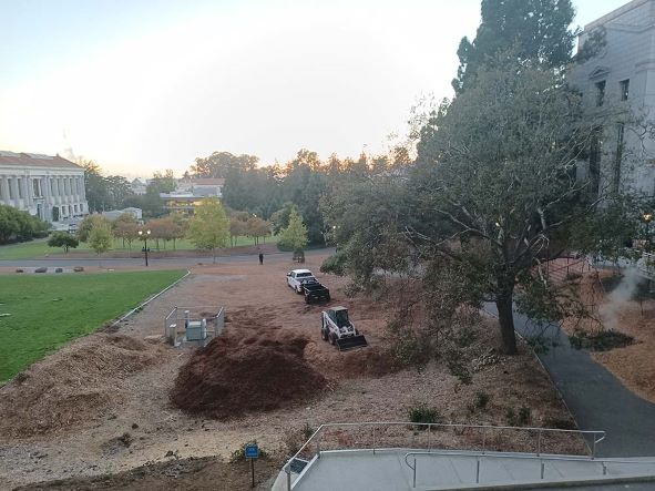
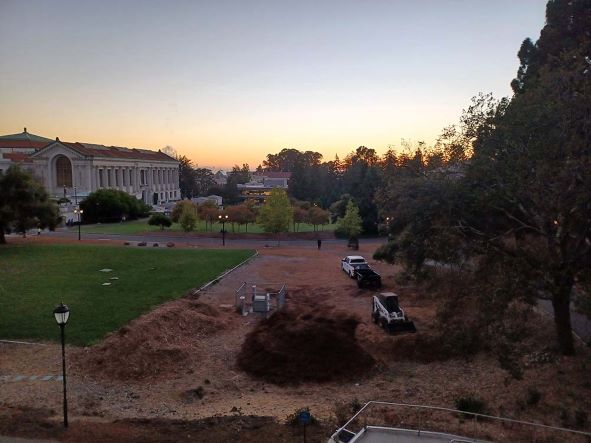
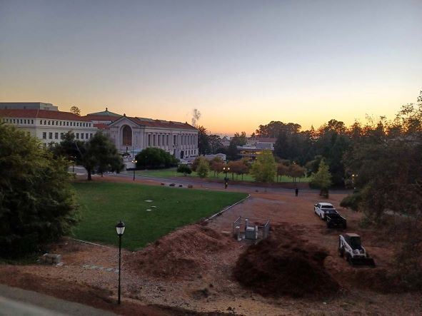
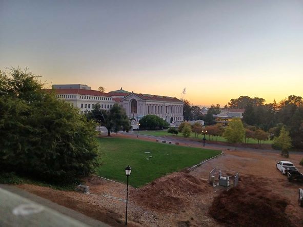
Here are all the raw pictures I took for this assignment:
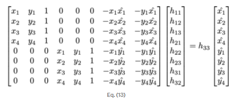
To compute the homography transformation matrix from one set of points into another, I needed to set up a system of equations. Basically, I used equation 13 from here. To expound a bit upon it, we know that our homography should transform our points in the first image to points on the rays passing through the points in the second image and the focal point. However, we can't say where on the ray they'll end up. So we introduce a free depth variable z_a to account for this, but this means that there could be multiple matrices that transform the points onto different depths along the ray. To constrain the equation, we then fix h_33 to be 1. Then by subsituting in for z_a, we can remove it from the equation and instead get it in terms of h_33, which we already predetermined to be 1, as in equation 13. Finally, we can solve the equation using least squares.
To get the actual points for the homography computation, I used matplotlib's ginput. However, to help correct inaccuracies in my annotations, I use the pixel near my annotation with the greatest NCC instead.
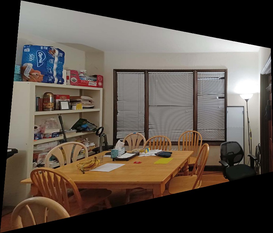
To rectify images, I computed the homography of a rectangular object in the picture onto a rectangle on the image plane. To determine the size of the output image I computed the range of the transformed corners of the original image. Then I used inverse warping to fill in the output image.
|
|
|
|
|
|
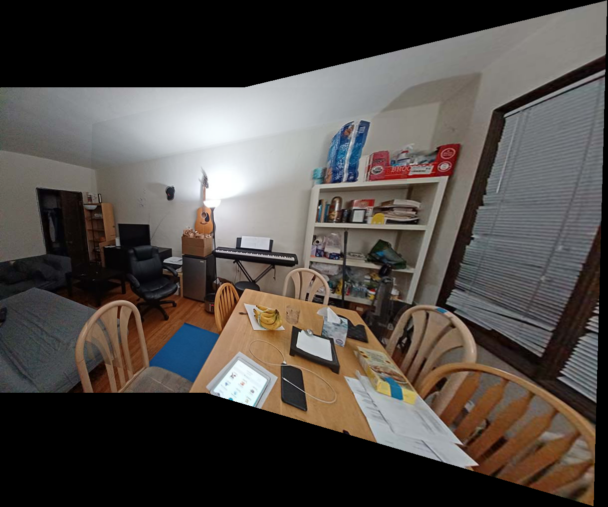
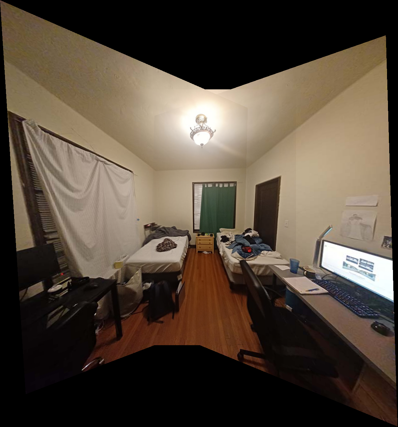
To blend multiple images together, I would iterate through each image and warp them all into the first image's plane. With each new image, the output mosaic would grow. I had to keep track of how the original image plane was shifting w/ respect to the image indices as a result of expanding the image. To blend the images together, I weighted each pixel's contribution by a ramp/pyramid that had a weight of 1 at the center of the warped image and 0 at the furthest corner, and at the end, I would divide by the sum of the weights across iterations. In addition, I also had to keep track of out of bounds pixels in the output mosaic. To account for this, when I compute sum of weights, I only use the weights at non zero pixel values. After iterating through the images, for pixels with 0 total weight, I instead set the weight to infinity, so that pixel becomes black on the final output.
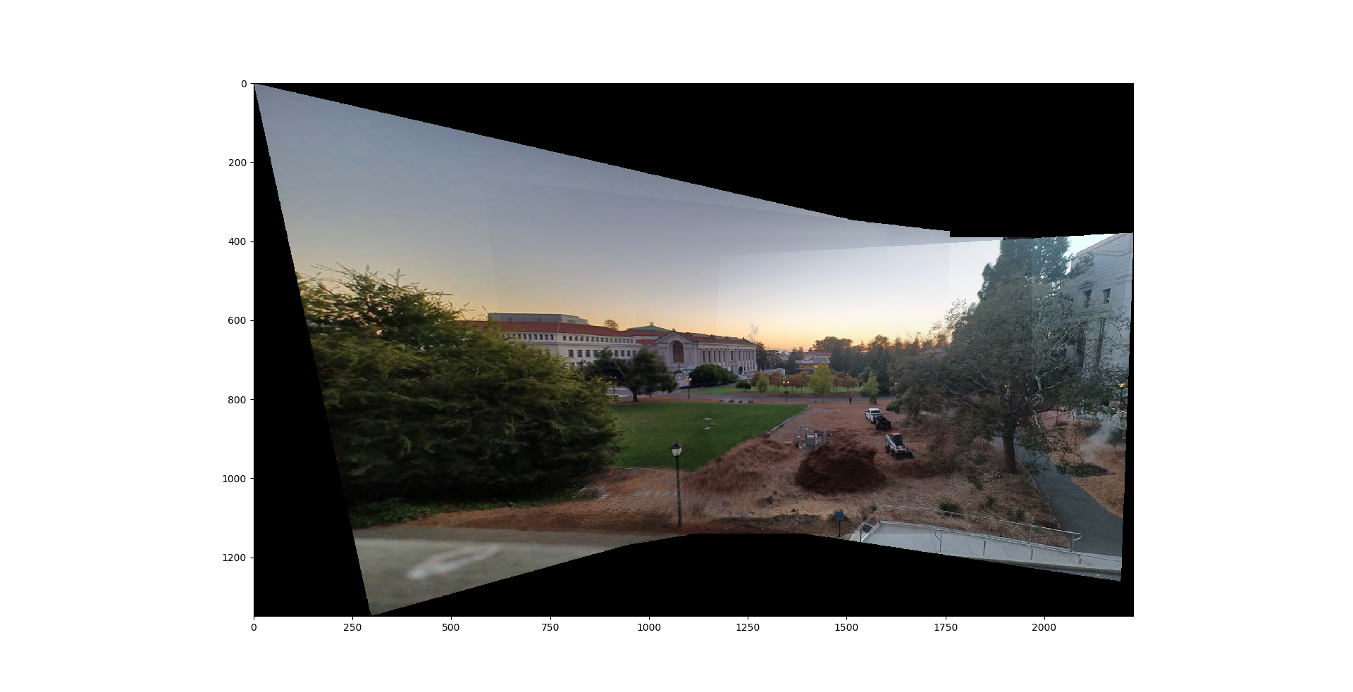
As a note, I accidentally took one of the pictures in the glade mosaic with a different lighting setting, so it makes the edge stand out
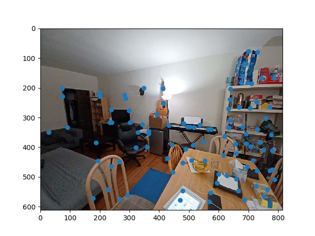
In this portion of the project I used the Harris Interest Point Detector to find interest points, adaptive non-maximal suppresion to select the best interest points, Multiscale Oriented Patches to compute features at each interest point, Lowe thresholding to select corresponding interest points, and RANSAC to remove outliers. Finally, I used these correspondes to once again produce a mosaic, as in part A.
To find interest points, I simply used the provided harris detection code and chose a corner strength threshold of .1 .
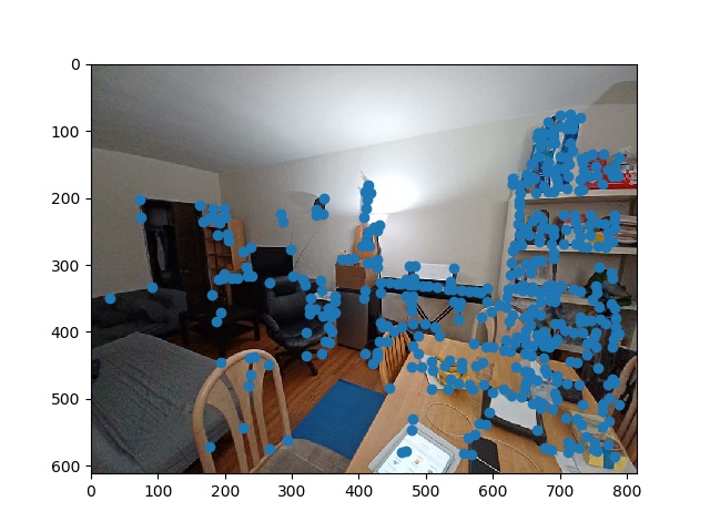
Non-Maximum Suppression (NMS) involves taking the point with the highest corner score, removing all its neighbors in a given radius, finding the point with the next highest score among the remaining points, removing all its neighbors, and repeating until no points are left. It ensures that the interest points are well spaced and correspond to different features in the image. Adaptive (NMS) produces a fixed number of points by searching over the suppression radius until the desired number of points is found. In practice, I instead computed the minimum suppression radius for each point given by the following equation

and sorted according to that radius. Then I took the k points with the largest suppression radius, where k is the number of interest points I desired.
To compute features, I used Multiscale Oriented Patches (MOPS) as described in the paper. For each interest point, I took a 40x40 window around it, applied a low pass filter, and then downsampled it to an 8x8 patch. Finally I flatted and normalized the resulting feature so be 0 mean and variance 1.
To match features, I used the Lowe approach described in class. For my two set of features from each image, I computed the pairwise distance between them in the feature space. Then I took the smallest two distances for each feature in the first image and computed the ratio between the smallest distance and the second smallest. The points with a ratio below .5 were retained, and their correspondence in the second image was their closest neighbor in the feature space.

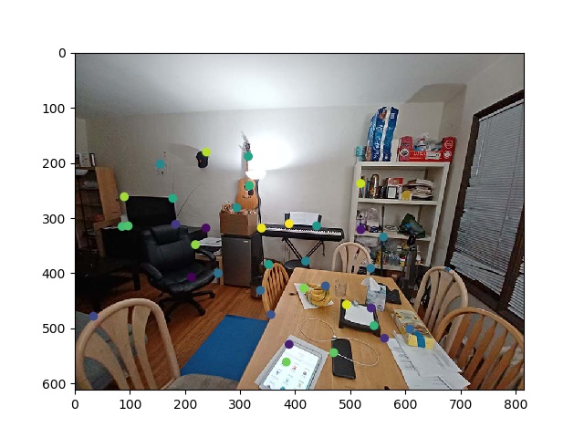
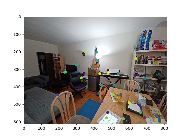
In the final step for computing correspondences, I used RANSAC to detect and remove outliers. RANSAC basically involves randomly selecting 4 proposed correspondences, using them to compute a homography matrix, and seeing if the other points agree with their homography. This is repeated until a homography is found with a large enough consensus (a sufficient number of inliers). The homography matrix is then recomputed using all these inliers. In the images below, you can see that the top left corner of the door frame, which was previously matched to the top left corner of the TV, has been removed after RANSAC.

Here I compare the mosaics formed from automatically generated correspondences with those from Part A, where I selected correspondences by hand. Automatic results are the right, hand picked results are the left. The results are surprisingly good!