CS194-26 Project 4B: Auto-Stitching Mosaics
Rishi Upadhyay, rishi.upadhyay@berkeley.edu, 3033975663
Project Overview
For this part of the project, we extended our system from last time to automatically find correspondence points and stitch images together.
Part 1: Detecting Corner Features in an Image
For this part, we used some given code to detect corner features within an image. As an example:
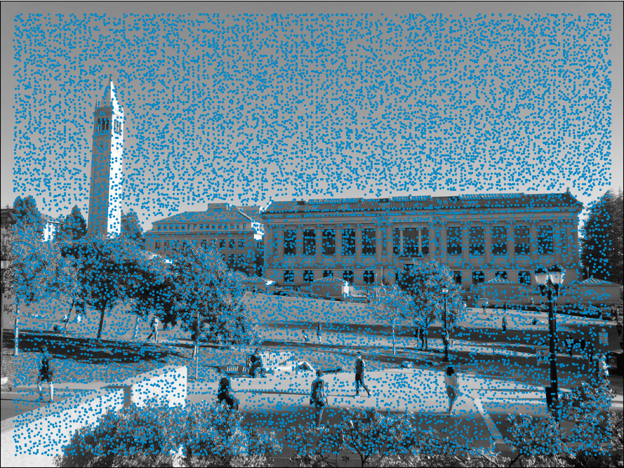
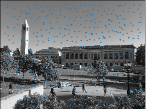
We then extended this using Adaptive Non-Maximal Suppression, a technique which filters out points by only taking strong corners and attempting to spread out the points throughout the image. After applying this technique, we chose to leave 500 interest points:
Part 2: Extracting Feature Descriptors
In this section, we extracted feature descriptors from the interest points we located in the previous part. What this means is that we extract an 8x8 matrix which contains pixels spanning a 40x40 region on the actual image. This is done to get a blurred, slightly more global descriptor.
After acquiring these, we normalize them to 0 mean and 1 std dev.
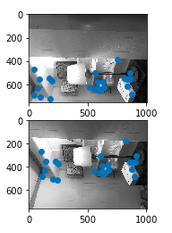
Part 3: Matching Feature Descriptors
After we acquired our feature descriptors, it was important to match them across images. To do this, we use the provided dist2 function. This gives us the Euclidean squared distance between all sets of points. After we have matched points across the images, we have to take an additional step to remove bad matches. We do this by examining the distance to the first and second nearest neighbor. We divide D_1 by D_2, and make sure that the ratio is below a certain threshold. I found in practice that this threshold varied between images. Some images had similar landscapes for larger regions and therefore often required higher thresholds to work well while others had great detail and required small thresholds to make sure there weren't too many outliers.
Here is an example of feature descriptors remaining after thresholding:
Part 4: Use RANSAC to compute a homography
After we had found robust matches, we used RANSAC to compute a homography. The idea behind RANSAC is to throw out outliers by picking 4 random points, computing a homography, then testing how many points are transferred well by this homography. At the end of the iterations, you take the homography that transfers the most points well. In order to quantify how well a point is transferred, we take the distance between the point after applying the homography matrix and the corresponding point on the other image. We then compare this distance to an epsilon. Just like the thresholding, I found that this epsilon required adjusting depending on the images, but most of the time could be kept between 1-10 pixels.
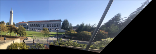
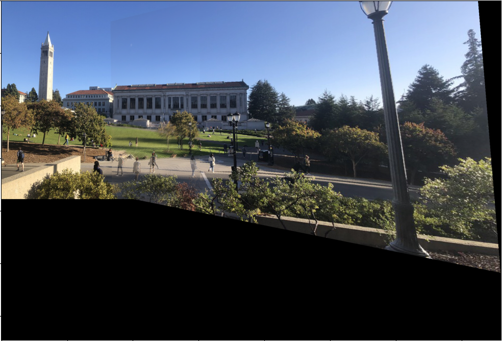
Part 5: Create Mosaics
Mosaic #1
Automatic & Manual
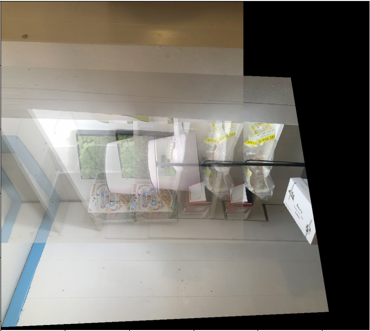
Mosaic #2
Failure Case - the threshold was too high
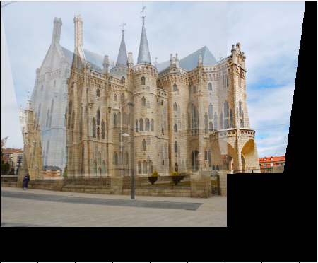
 Mosaic #3
 What did I learn
I learned how finicky this solution was and gained a new found appreciation for the human eyes and our visual systems abilities.
What did I learn
I learned how finicky this solution was and gained a new found appreciation for the human eyes and our visual systems abilities.