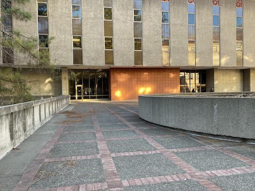
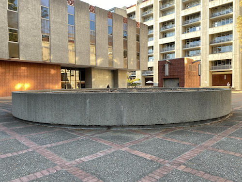
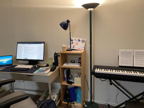
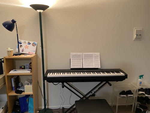
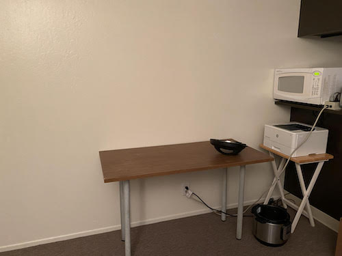
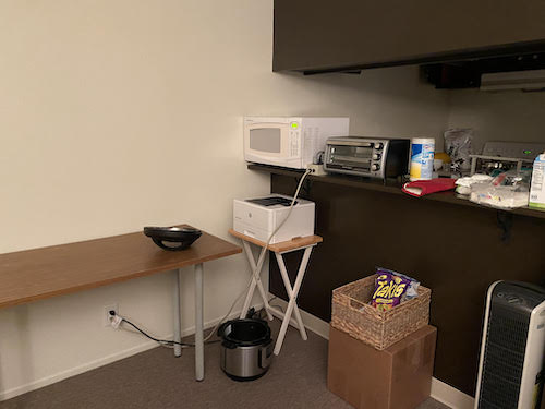
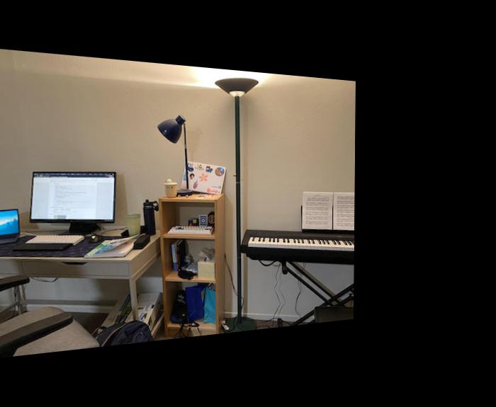
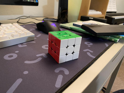
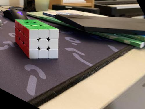
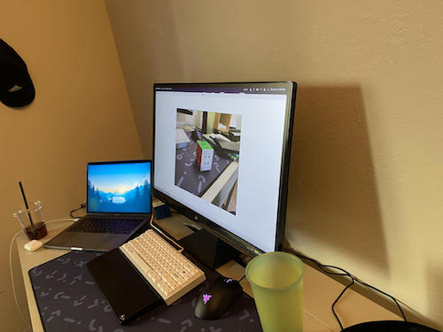
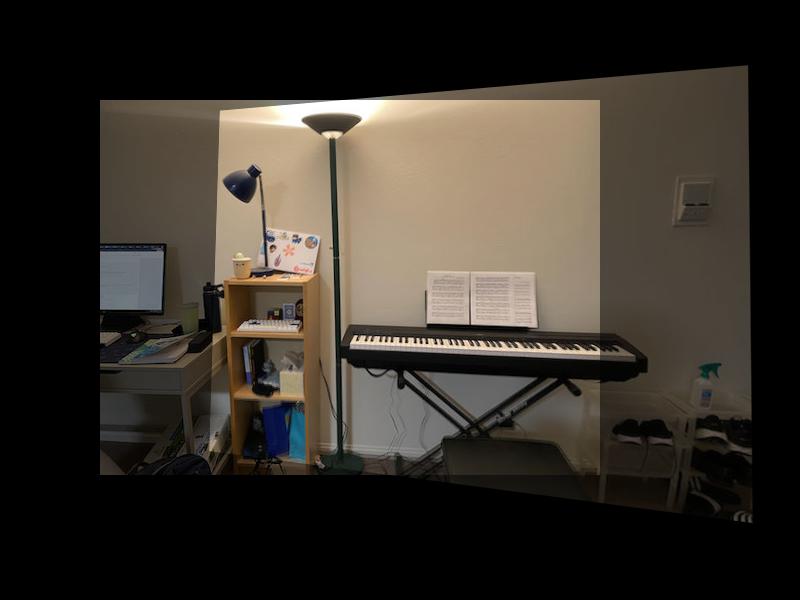
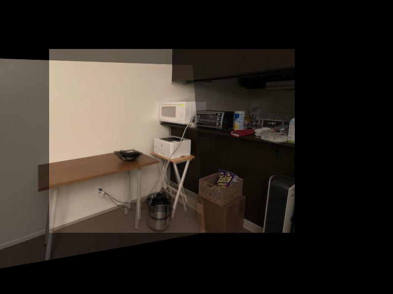
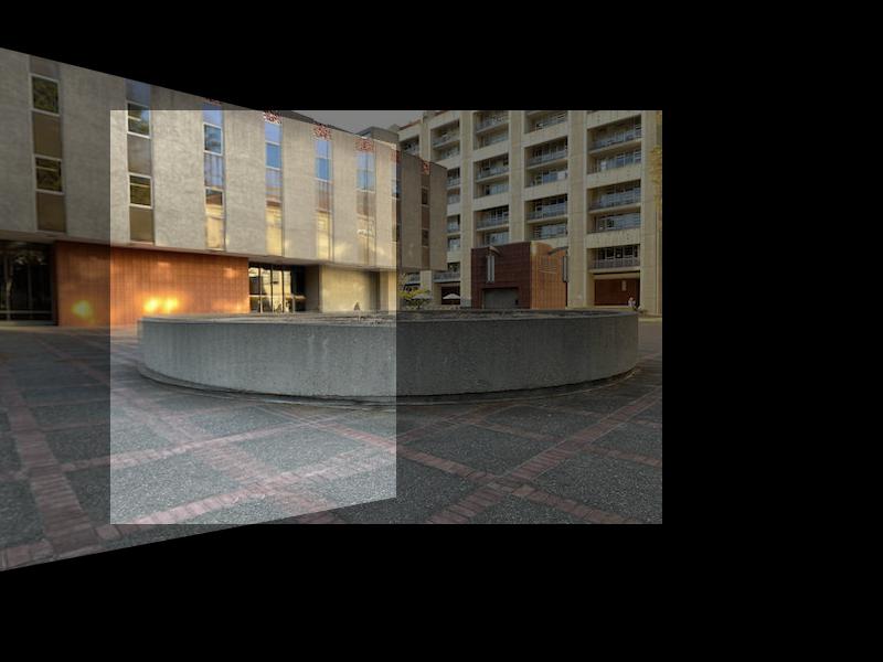
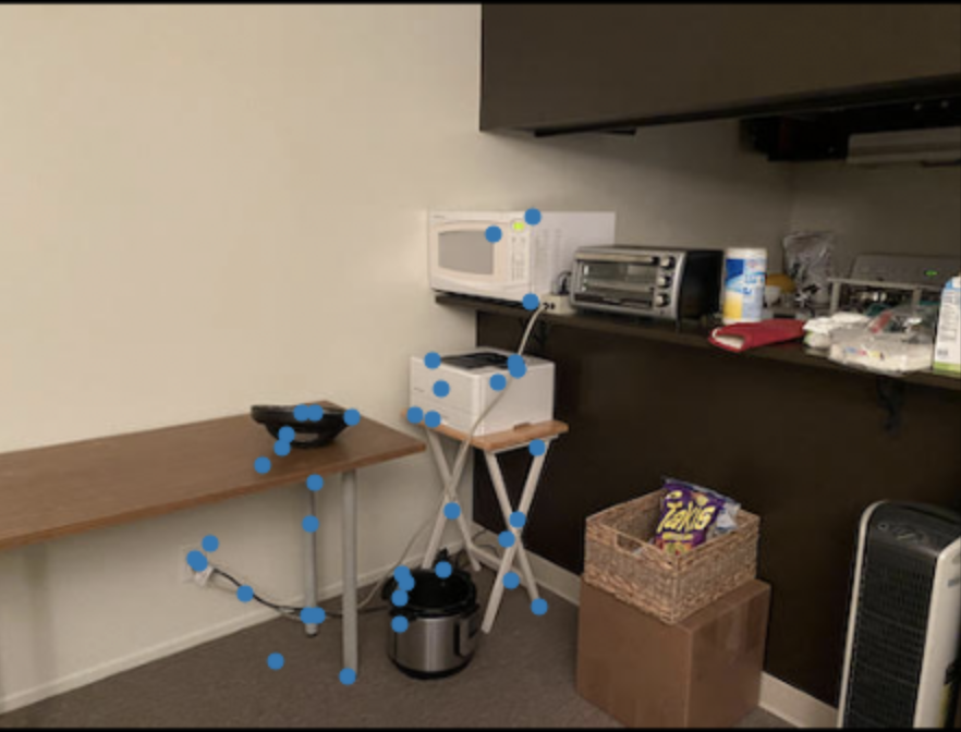
Displayed below are the photos that will be warped and blended together.
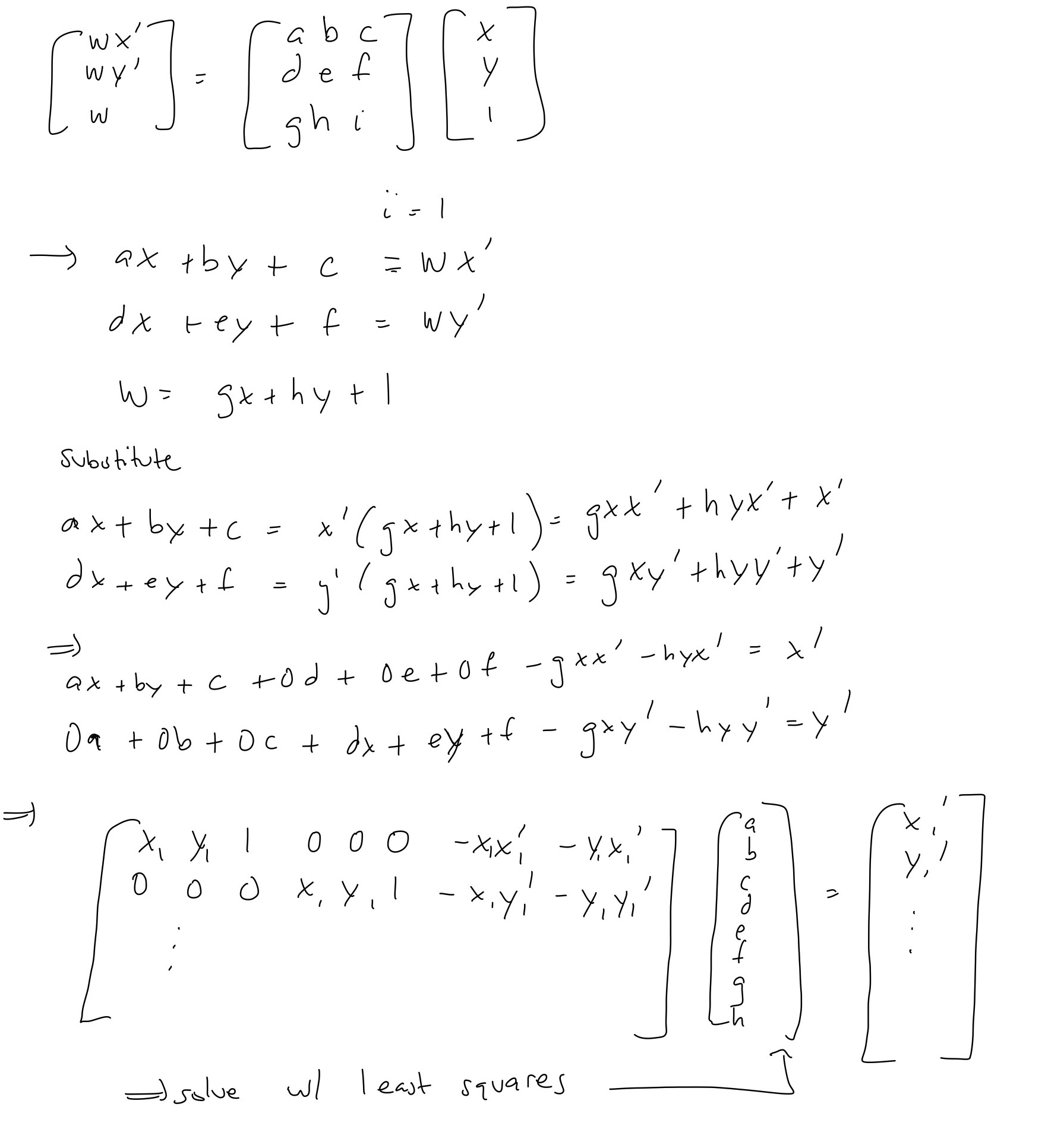
In this we want to find a homography H that will transform the image so that we can warp the pespective to match the target image. To do so, we setup a system of equations, giving us an overconstrained system which we can solve with least squares. I show the setup below. For each pair of images, I selected 10 correspondence points at corners.
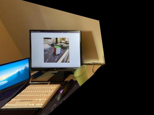
After recovering the homography, I use linear interpolation to warp the image perspective. In the target image, we search for the corresponding point in the source image and interpolate the pixel value similar to project 3.
In this part, I test our homography and warping functions by warping square and rectangle planes to be frontal parallel. We do this by selecting the corners of the plane as well as creating artifical points for frontal parallel plane.
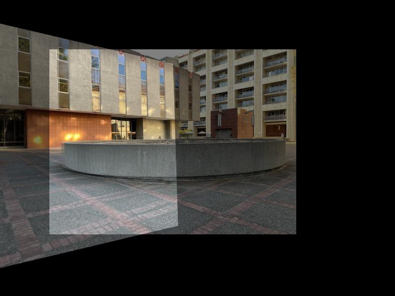
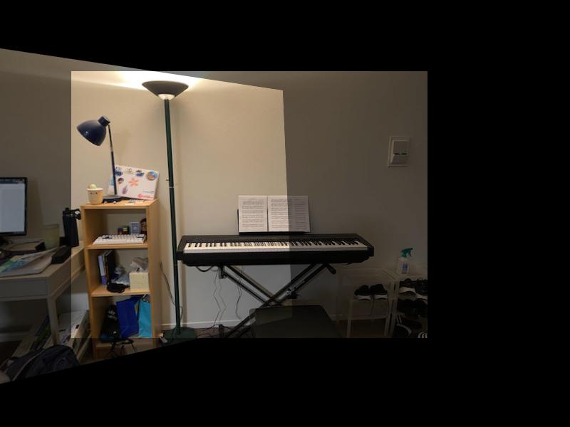
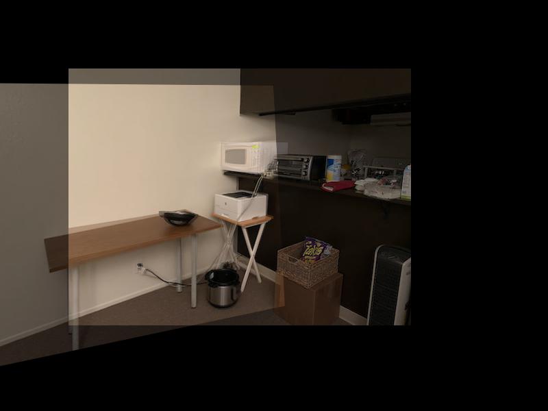
In this part, we blend the image together to create the final mosaic image.
It was very cool to be able to walk through the actual computation, mathematics, and process behind how panoramic photos could be made by warping perspectives and stitching images together. I learned that point correspondence are important and creating a clean mosaic image is difficult and requires a lot of extra image processing! It was also very cool to see how much information could be recovered by warping the perspective of the image!
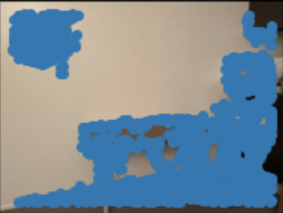
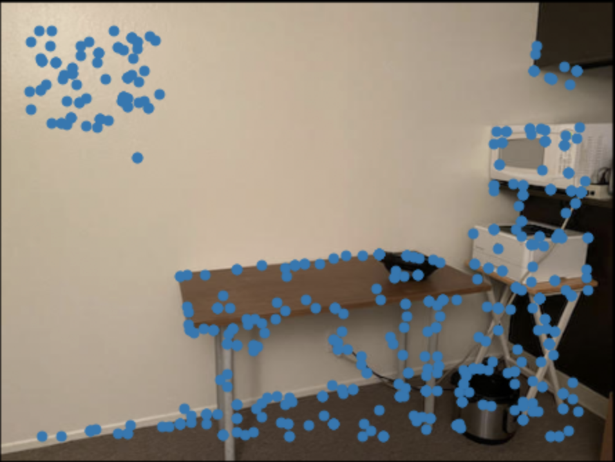
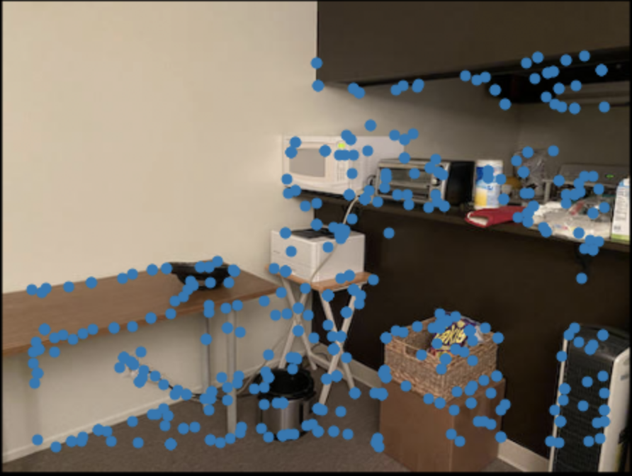
In this part, we use the harris detector to detect corners in the image where the gradient in all directions is significantly large. There are many points returned in this point and in the next few parts, we will filter them out. We use the same pictures as in Part 1. Check above for the originals.
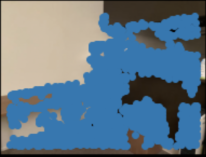
In this part, we use adaptive non-maximal suppression in order to find points with the strongest corner strengths while keeping the points well distributed across the image. We do this following the steps below.
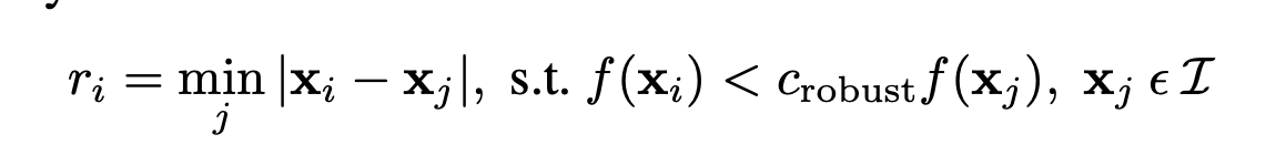
For each point in one of our images, we compute the minimum suppression radius using the formula shown above by computing distances to all other points satisfying the condition. We then take the highest 500 radiuses and use these points. We show the selected points below.
In this part, extract feature descriptors from the area surrounding each point. We sample from the 40x40 patch around each point, and by taking averages of 5x5 patch to end up with an 8x8 patch representing the feature descriptor. We use this in the next part for feature matching. We also make sure to normalize our patches to have mean 0 and std 1.
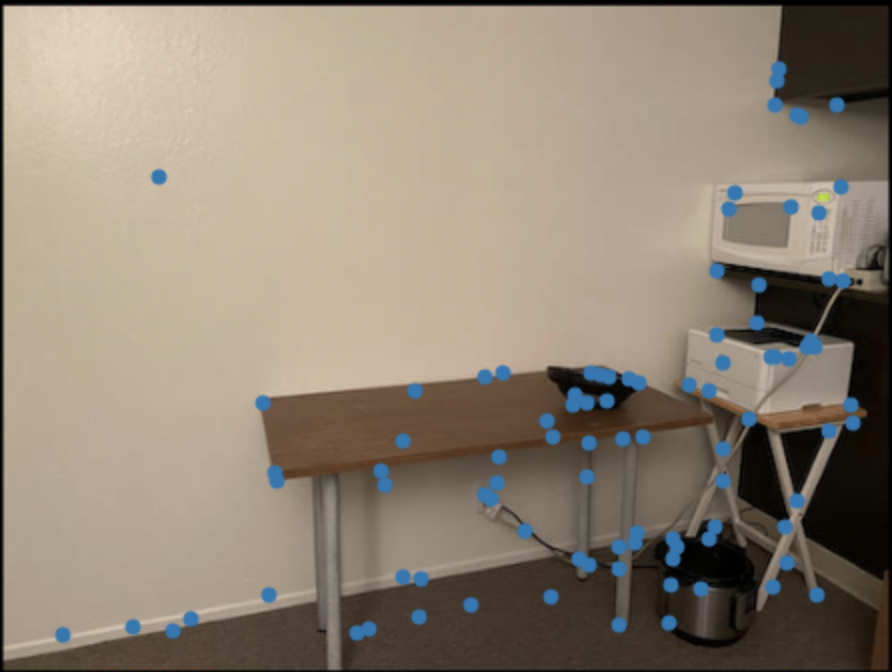
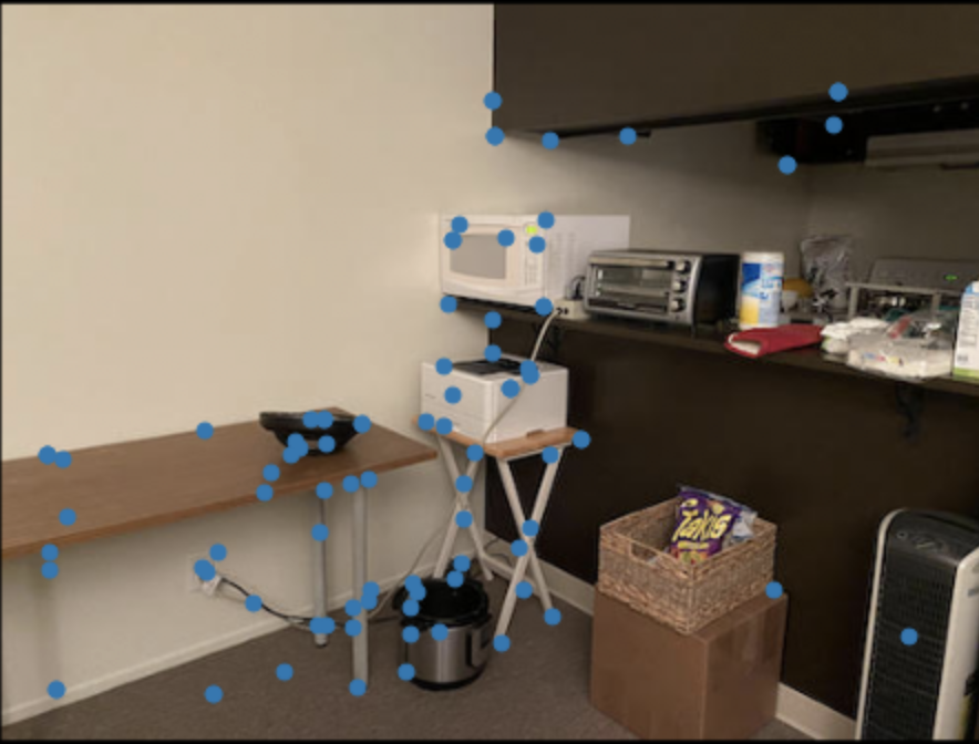
In this part, we run an kNN algorithm to find the feature matches across two images. For each feature descriptor in one image, we compute the error via SSD between all the feature descriptors in the other image. We take the feature descriptor with the lowest error as the feature match (the nearest neighbor). However, we use Lowe's method to filter out outliers or nonmatches. We only count it as a feature match if e_1/e_2, the ratio between first and second lowest errors is below a certain threshold epsilon which I choose to be 0.68 based on the graph in figure 6b of the MOPS paper. The reasoning is that if this was truly a match the highest error should be significantly lower than the next highest error. Below we show the selected feature correspondences.
In this part, we run the Ransac algorithm shown below which helps filter out outliers and non matches and helps us select a final set of corresponding feature points.
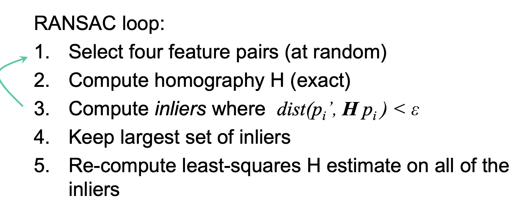
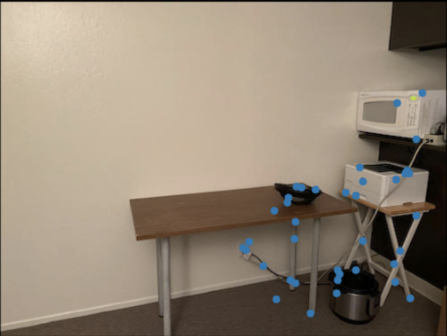
For a certain amount of iterations (I chose 1000), we select 4 random points, compute the homography, then compute the distances between the first image's points warped into the second image's perspective. We compute the distances (which can be thought of has perhaps errors) and we select all the points with low enough distances, we call these 'inliers'. We use the biggest set of inliers. This helps filter outliers even more. Below we show the results of ransac. The point correspondences which much better than the previous step which still had outliers.
Below we compare the manually and automatically stitched mosaics using the same images from part 1. Top is the manually stiched result. The bottom is the autostitched result.
I thought it was super cool to be able to run non machine learning algorithms to automatically detect significant feature points as well as select a strong, distributed set of feature points all automatically.