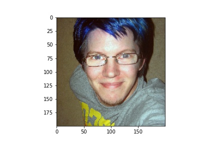
Part 1: Nose Tip Detection
To calculate the nose positioning of each image, we use a convolutional Neural Network (CNN). After iterating through multiple designs, I finalized with this structure:
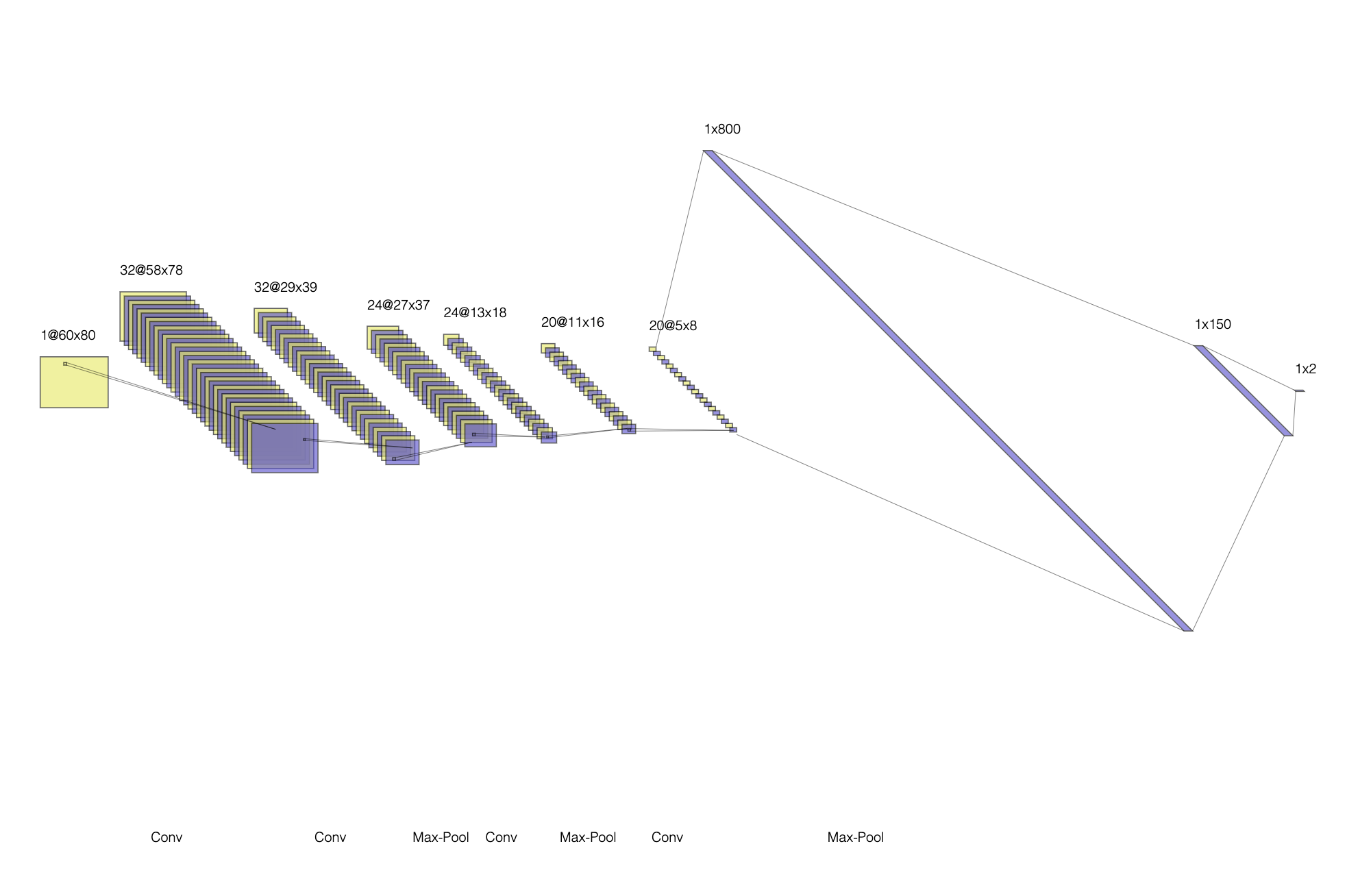
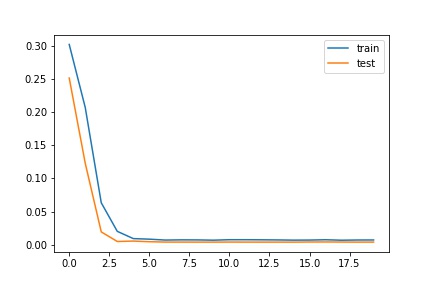
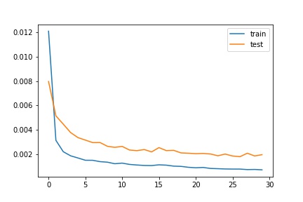
Running 25 epochs with a learning rate of 1e-3, the best test loss was 0.00188. Plotting the training resulting:
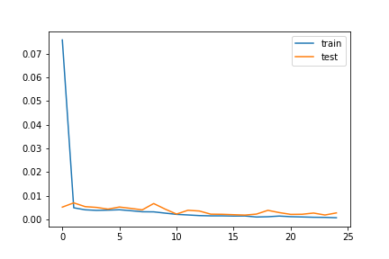
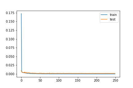
However, I had better results with the learning rate at 3e-4. I believe with the learning rate lower, the model trained slightly slower, but was able to reach a lower minimum through gradient descent. The best testing loss was 0.0013:
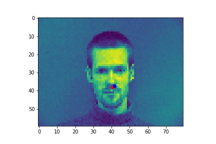
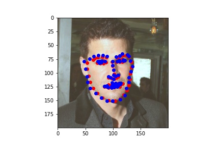
Nose Detection Results
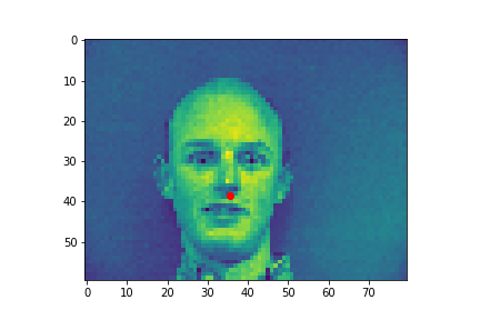
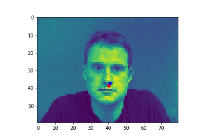
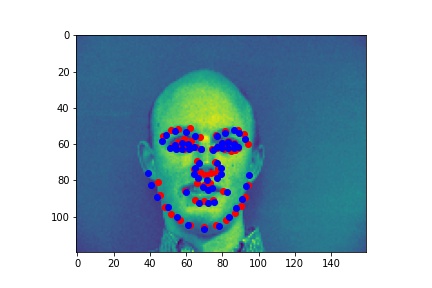
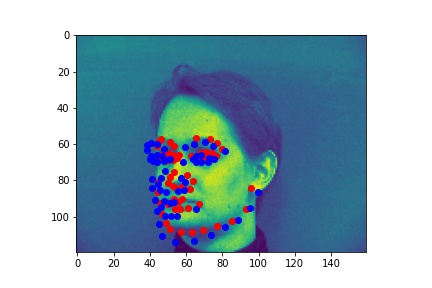
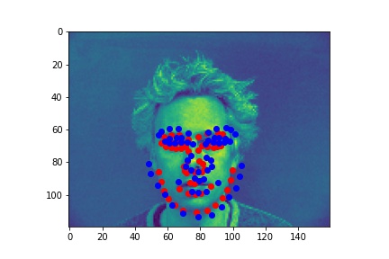
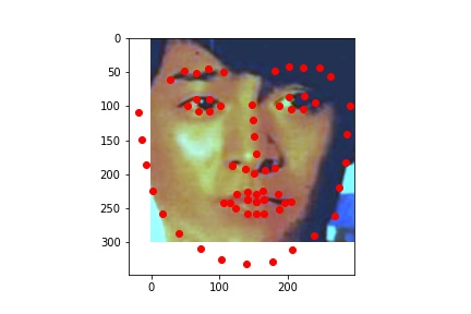
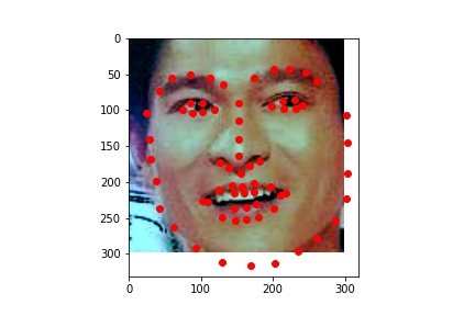
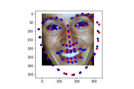
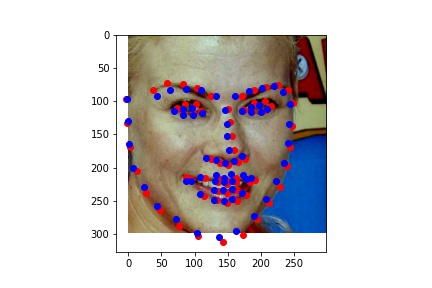
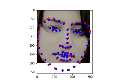
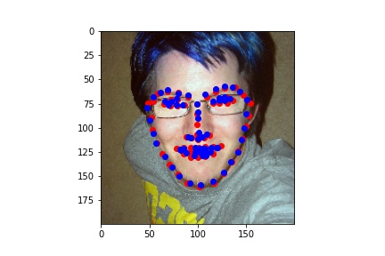
Red is ground truth, and blue is the output from the CNN.
Successes:
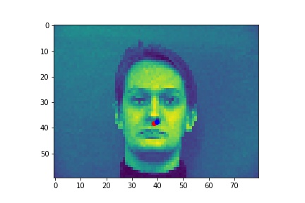
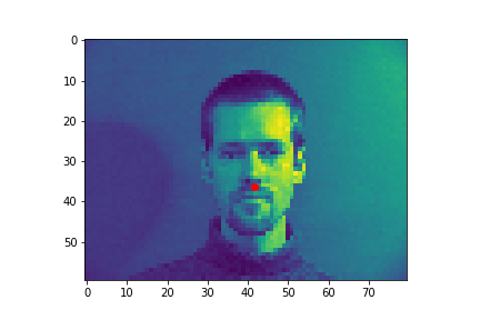
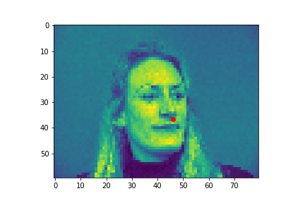
Failures:
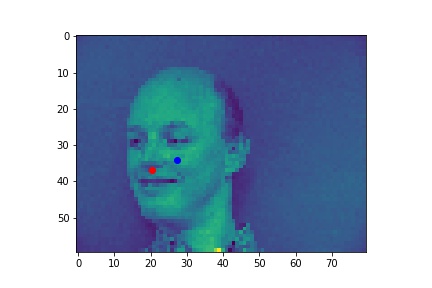
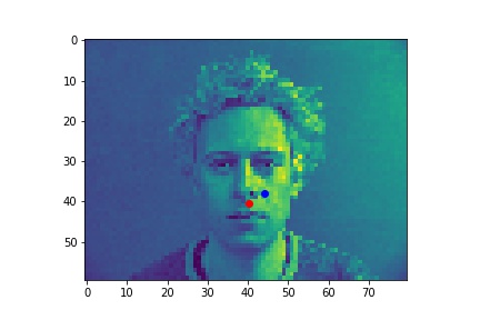
In the first case, the model may be confused, as the majority of the models show the face looking directly forward. It also has very low contrast, which may not give the model must signal to go by. In the second failure, the face is being lit from the right, which is not as common either.
Part 2: Full Facial Keypoints Detection
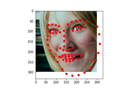
Here are some images and ground truth labels without augmentations:
With augmentions (color jitter, rotation, flips):
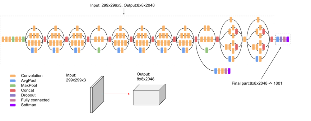
For full-face keypoint detection, a larger model was used:
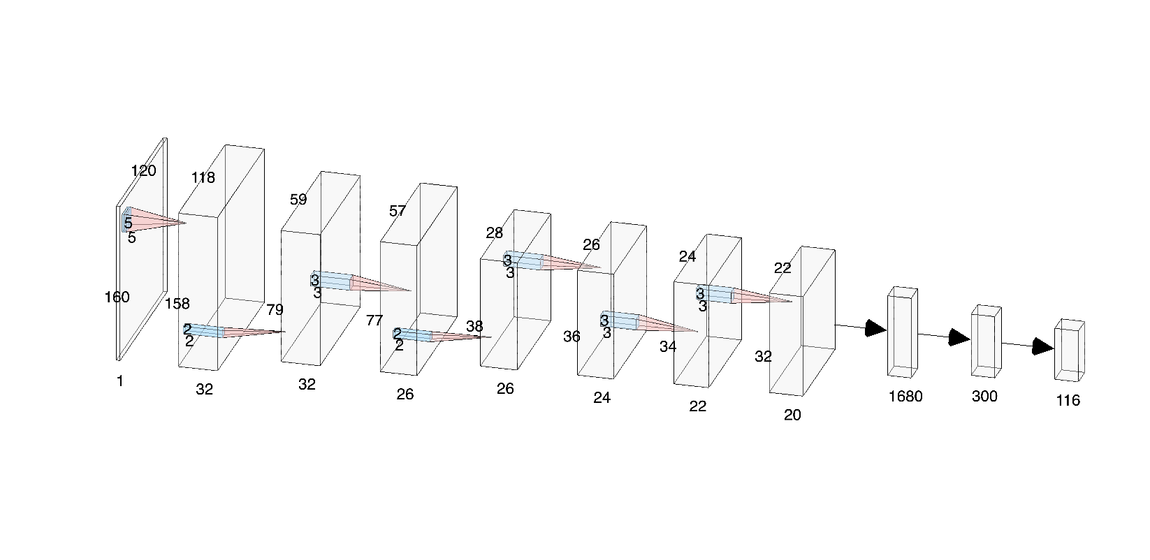
The model is composed of 2 convolution / max-pool blocks, then 3 convolutional blocks. The output is then flattened, then a 1000-node fully connected layer, and then a 300-node FC, finally with an output of 68 2-dimensional points. I messed around with different number of max-pool layers, but cut it down to 2 as the final output was getting too small to have any significant information.
This plot was over 20 epochs with a 3e-4 learning rate. I then copied the model and retrained from that and ran another 100 epochs at a smaller learning rate of 1e-4. I varied with batch size as well, ranging from 4 to 16, ultimately landing on 8 for all of training.
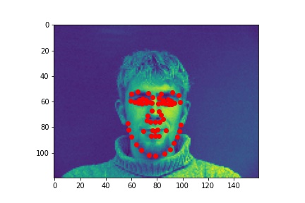
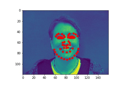
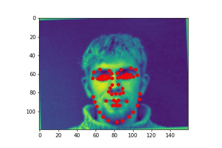
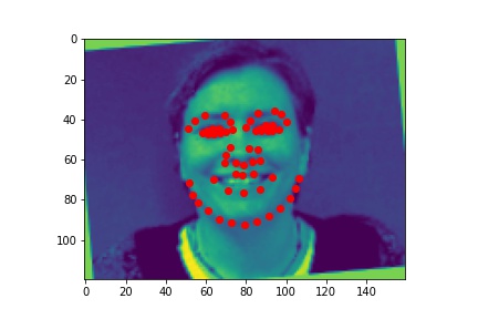
Successes:
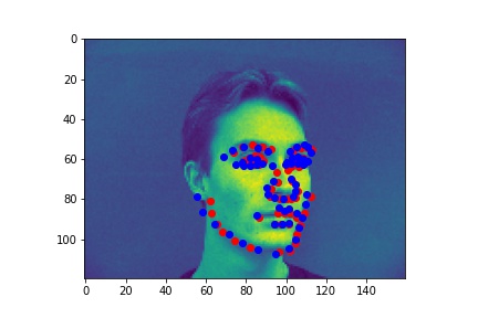
Failures:
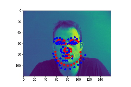
The model seemed to do well when there were sharp distictions between the different body parts. For the first image, the face was half in shadow, meaning there was low contrast over the neck-chin region. It does get the general area though, I just think by the end of the model, the features are so complex it has a hard time exactly placing them in the image. The last failure image had low contrast between the ears and the chin/neck, so it was not able to accurately differentiate between them.
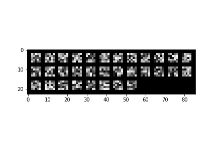
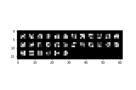
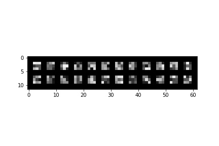
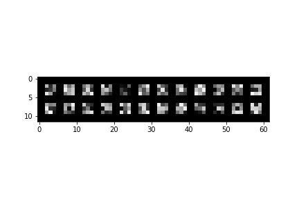
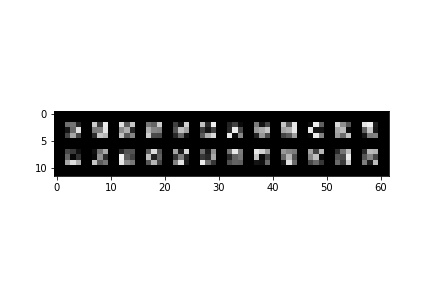
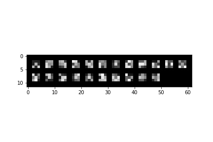
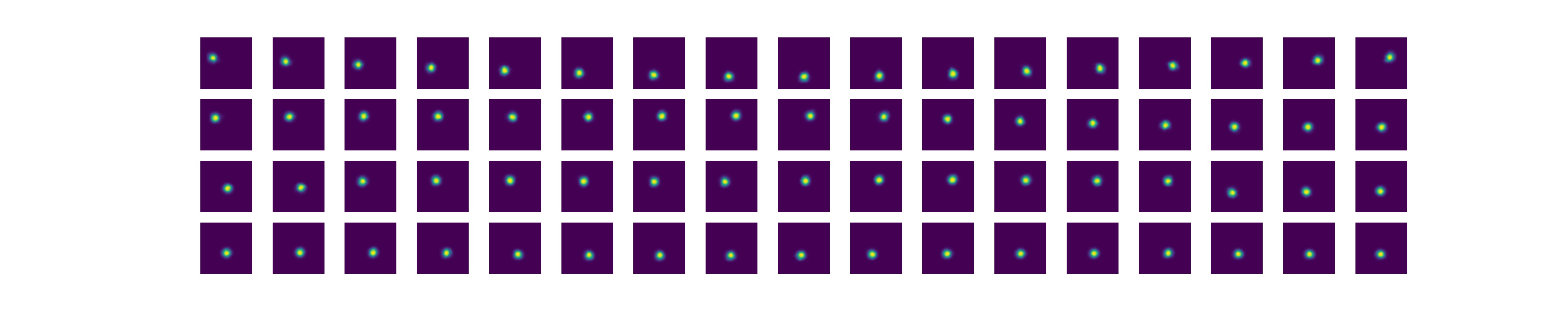
The filters of the network:
Part 3: Train With Larger Dataset
For Part 3, I used a variety of different pretrained models as a backbone. I would plug-and-play different models, then change the final layer of the pretrained model to be a fully connected layer of size 200, then added another fully connected layer the size of the output-- 68 * 2 = 136.
For the backbone, I tried Resnet18, Resnet34, Resnet50, and Resnet152. Out of those, I had the best results with Resnet34 and Resnet50-- I believe this was because the larger resnets were just too deep and overfitting to the training data. After Resnets, I tried another type of pretrained model: Inception_v3. The model is usually used for image classification, but seemed to do fairly well plugged in place with a couple additional FC layers.
With the Inception v3, I was able to get a score of 7.92233 on Kaggle! I decided not to go through with data augmentation in this case, as there seemed to be enough training data already, and my inception model was not overfitting significantly. Batch size was 16, and learning rate was set to 1e-3 for the first 15 epochs, then brought to 3e-4 for the last 15.
Training / Validation Error Graph:
Data from the dataloader:
Model Outputs from Test Set:
My Results:
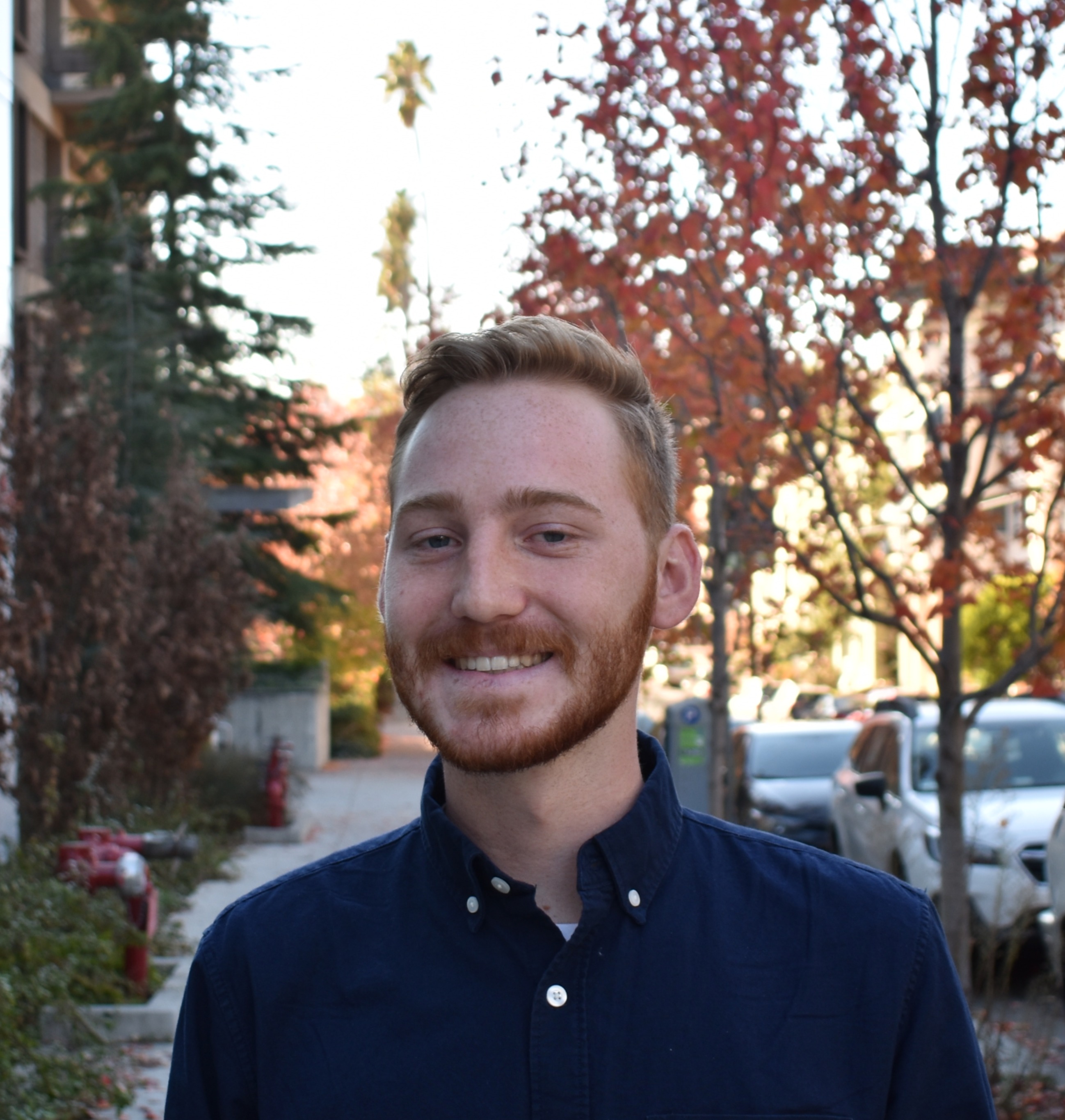
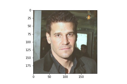
For my results, I picked two images of myself, and one of my friend Aaron-- these images are similar to those that were used for Project 3 warping:
Originals:


Model Results:
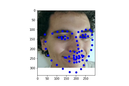
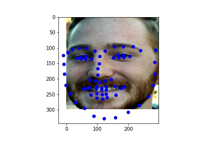
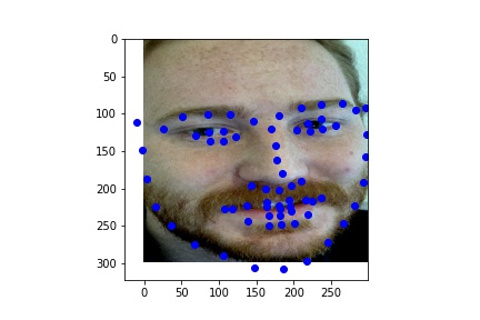
Overall, this model did fairly well on images not from the original training or validation set. There are only minor mistakes due to the beard and mustache, as that was not representated well enough in the training data.
Bells and Whistles: Gaussian Heatmaps
To convert the problem from above into a heatmap problem, it required a different network and new labels.
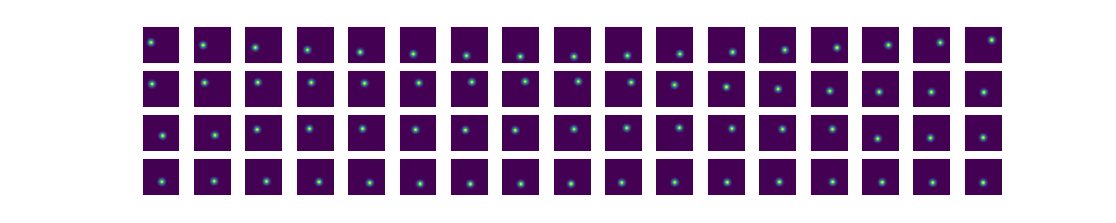
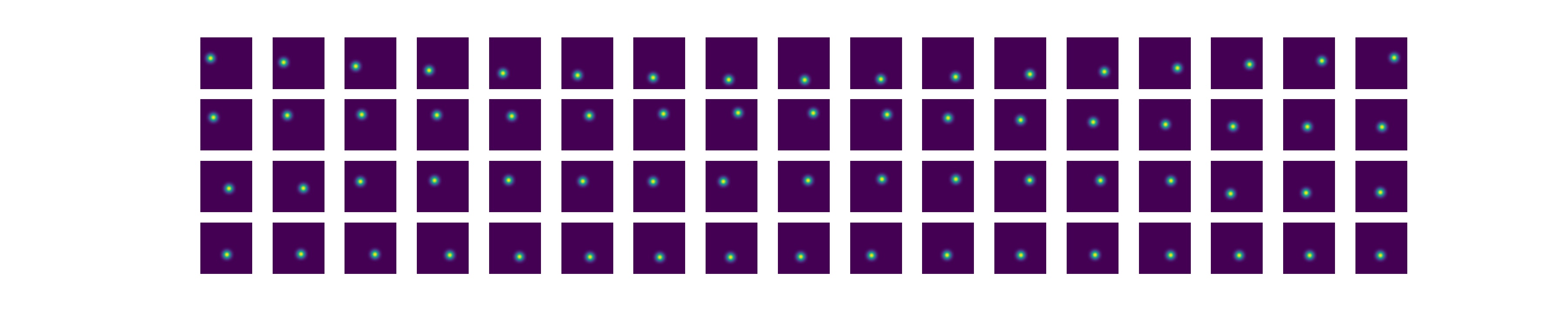
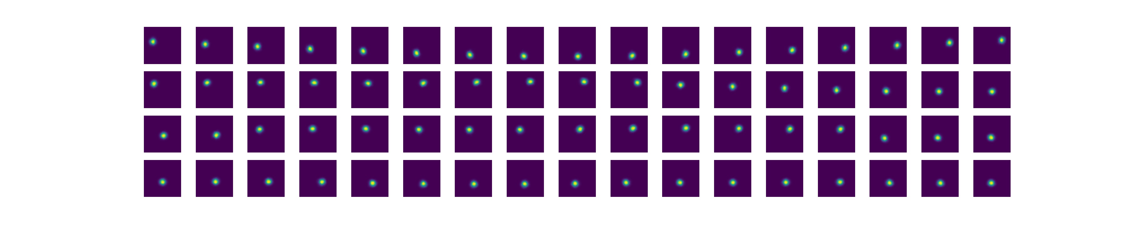
The Labels
Labels were created by getting each ground truth keypoint, and building a 200x200 image from them, where at the keypoint, a unit gaussian is placed. This was modeling each pixel almost like a class of its own-- each was a bernoulli random variable with some probability of being the keypoint. To get the final outputs, you just pick the maximum value out of all those classification probabilities.
I had to change the labels slightly from the previous question, as a lot of keypoints in the previous question were outside the bbox bounds given by the dataset. This posed a big problem for labeling, as then I would never be able to capture the argmax index to put the keypoints. I tried to first fix this by making the labels the whole image, disregarding the bounding box, but that proved either too memory intensive, or not exact enough when scaling down to an appropriate size.
Storing 68 separate 200x200 labels was pretty expensive, so I needed to keep batch size low for most of training.
The Model
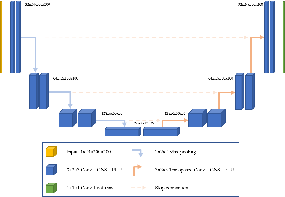
For my model, I used a modified U-Net, heavily based off of this repo: (https://fairyonice.github.io/Achieving-top-5-in-Kaggles-facial-keypoints-detection-using-FCN.html) This is a standard U-Net, where each down and upscale block is a double convolution with a relu in-between.
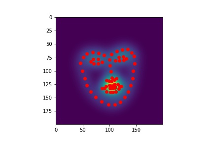
Results!
For image 5:
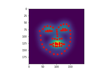
For image 500:
Overall, the heat map values seemed to do significantly better than the resnet/inception models at getting precise points, though it did take much longer to train as there was no pretraining involved.