Part 1: Nose Tip Detection
Part 2: Full Facial Keypoints Detection
Part 3: Train with a Larger Dataset
The goal of this project is to automatically detect facial keypoints with a deep convolutional neural network (CNN). To train and validate our networks, we will use the IMM Face Dataset for Parts 1 and 2 and the iBUG Face Dataset for Part 3.
For both Part 1 and Part 2, we will use the IMM Face Dataset which contains 240 facial images of 40 persons; each person has 6 facial images in different viewpoints.
We will use the first 32 persons' images (32 x 6 = 192 total images) for the training set and the last 8 persons' images (8 x 6 = 48 total images) for the validation set.
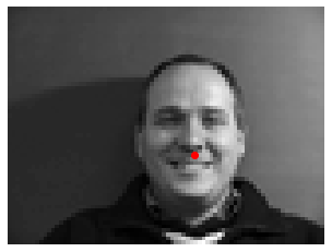
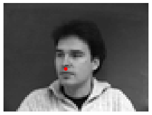
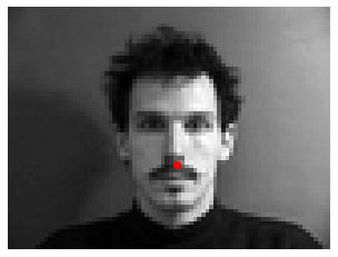
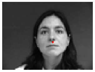
Let's first visualize our data and nose keypoints. The images are resized to 80x60 and converted to grayscale.
Here a few of the samples with their ground-truth nose keypoints.
We will now define our convolutional neural network (CNN).
I used 3 convolutional layers (torch.nn.Conv2d),
each followed by a Rectilinear Unit (ReLu) layer (torch.nn.ReLu) as non-linearity and a max pooling layer (torch.nn.MaxPool2d) of size 2.
Then, this is followed by 2 fully connected layers (with a ReLu layer in between).
NoseKeypointNet(
(conv1): Conv2d(1, 16, kernel_size=(3, 3), stride=(1, 1))
(conv2): Conv2d(16, 32, kernel_size=(3, 3), stride=(1, 1))
(conv3): Conv2d(32, 64, kernel_size=(3, 3), stride=(1, 1))
(fc1): Linear(in_features=2560, out_features=256, bias=True)
(fc2): Linear(in_features=256, out_features=2, bias=True)
)
With this network, we can start training the CNN and predicting keypoints.
We will use mean squared error (MSE) loss (torch.nn.MSELoss) as the prediction loss and train the CNN using Adam (torch.optim.Adam).
Tweaking the hyperparameters (e.g. number of layers, channel size, filter size, learning rate) will produce different results.
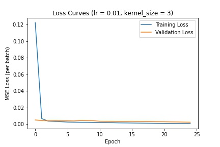
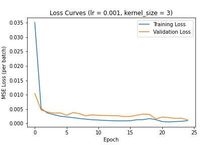
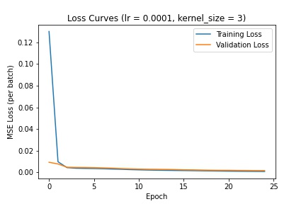
I used a batch size of 4, trained the network for 25 epochs, and tuned the learning rate and network's kernel filter size.
Here are the different loss curves for the training and validation sets when we change the learning rate:
Here are the different loss curves for the training and validation sets when we change the kernel filter size:
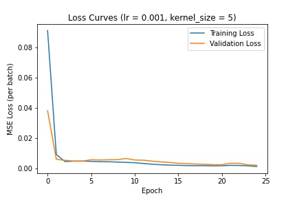
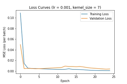
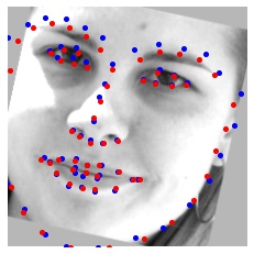
I decided to go with a learning rate of 1e-3 and kernel size of 3 (as defined in the above CNN). The following are several examples using this trained network to predict nose keypoints (predictions in blue, ground-truth in red):
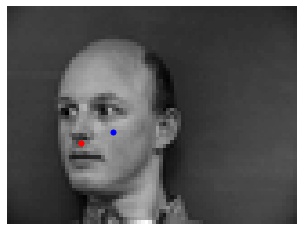
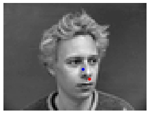
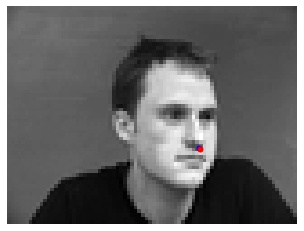
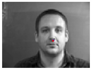
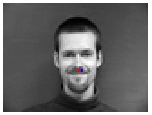
In general, the network predicted nose keypoints better for faces looking straight ahead than those turned to the side. This is probably because a majority of the training data was front-facing faces.
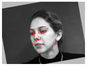
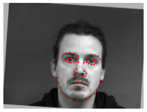
Now, we will detect all 58 facial keypoints.
Similar to Part 1, we will first load in our data and visualize it. The images are resized to 240x180 and converted to grayscale.
Since our dataset is small, we will need data augmentation to prevent the model from overfitting.
Data augmentation involves applying random transformations to the training data.
I chose to apply random rotations of -15 to 15 degrees, shifts of -10 to 10 pixels in both the x and y directions, and brightness changes.
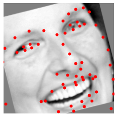
Below are several samples displaying the image and the ground-truth keypoints.
The CNN layers used for predicting facial keypoints is defined below. Each convolution layer is followed by a ReLu and max pooling layer, similar to the CNN in Part 1.
FaceKeypointNet(
(conv1): Conv2d(1, 16, kernel_size=(3, 3), stride=(1, 1))
(conv2): Conv2d(16, 32, kernel_size=(3, 3), stride=(1, 1))
(conv3): Conv2d(32, 64, kernel_size=(3, 3), stride=(1, 1))
(conv4): Conv2d(64, 128, kernel_size=(3, 3), stride=(1, 1))
(conv5): Conv2d(128, 256, kernel_size=(3, 3), stride=(1, 1))
(pool): MaxPool2d(kernel_size=2, stride=2, padding=0, dilation=1, ceil_mode=False)
(fc1): Linear(in_features=3840, out_features=256, bias=True)
(fc2): Linear(in_features=256, out_features=116, bias=True)
)
We will also train the network with MSELoss and Adam as we did in Part 1.
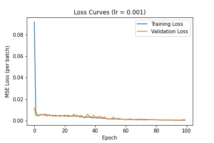
Below are the resulting loss curves for the datasets with batch sizes of 8:
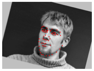
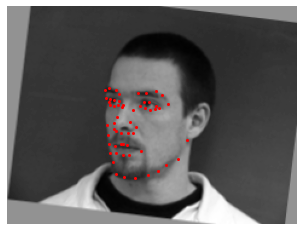
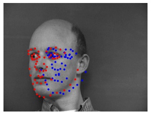
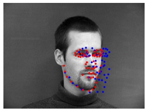
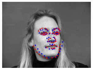
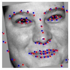
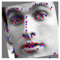
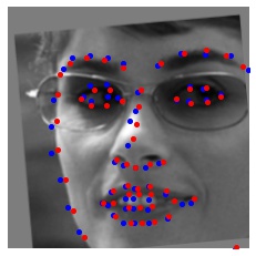
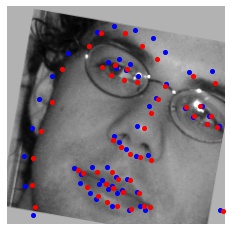
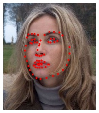
Here is a selection of the results, with predictions (blue) and ground-truth keypoints (red):
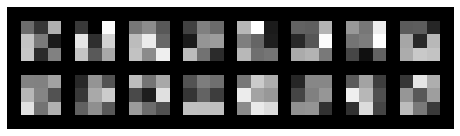
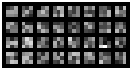
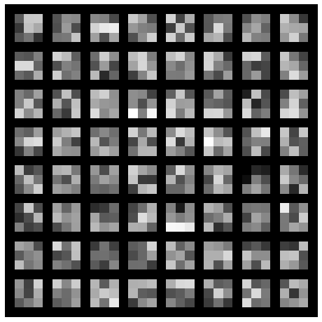
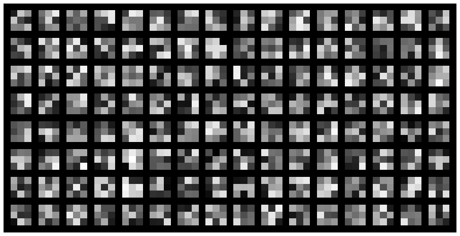
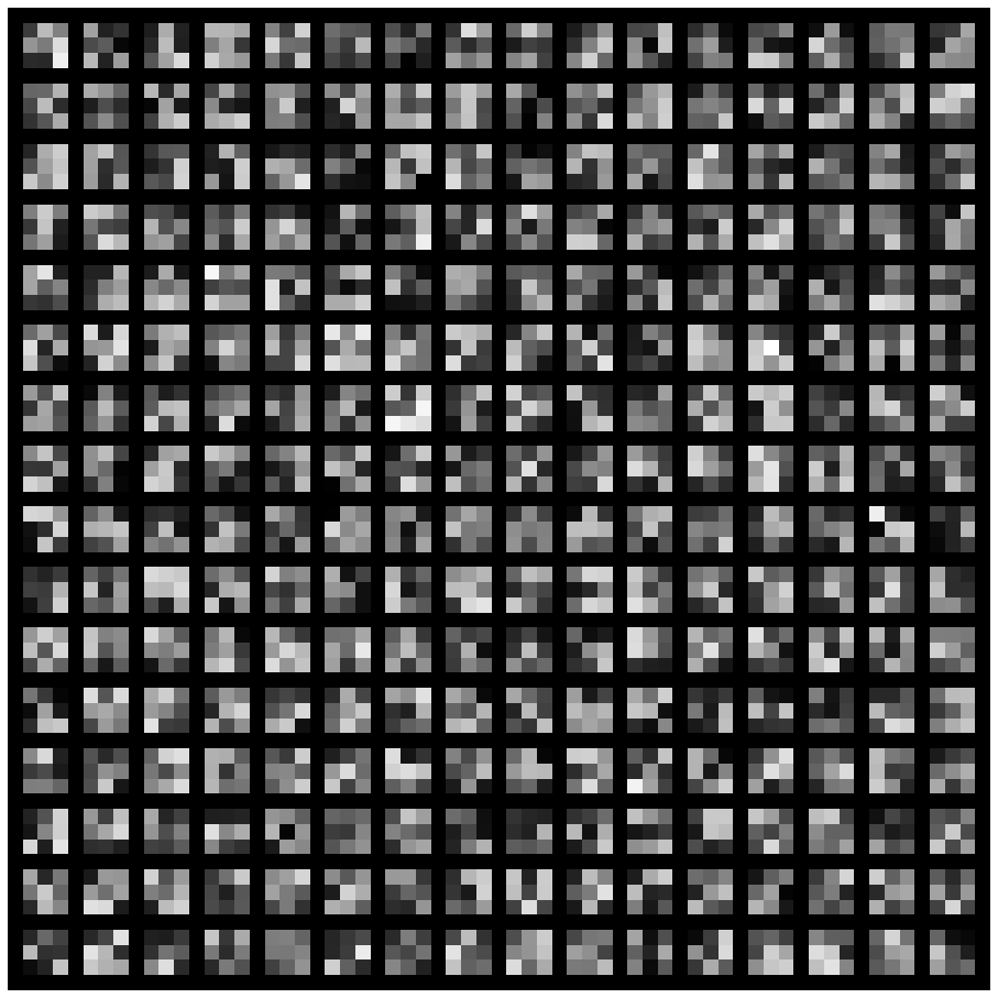
Let's also visualize our CNN's learned filters:
Now, we will train our network with the iBUG Face in the Wild dataset, which contains 6666 images of varying sizes and 68 annotated facial keypoints per image.
With each image in the dataset comes a bounding box generated by dlib's default face detector.
We will use this bounding box to crop the images so that the images we train our network on only include the faces.
Then, we resize the images to 224x224 and convert them to grayscale.
Similar to Part 2, we will use data augmentation, such as random rotations, shifts, and brightness changes, to prevent overfitting.
The dataset is also randomly split 80% into a training set and 20% into a validation set.
Here are several samples with their ground-truth keypoints:

The network we will use will be a pre-trained ResNet18 model (torchvision.models.resnet18)
that we modify to take in grayscale images and output 136 prediction values (68 keypoints * 2 (x and y coordinates)).
Below are the details of the model architecture:
iBugFaceNet(
(resnet18): ResNet(
(conv1): Conv2d(1, 64, kernel_size=(7, 7), stride=(2, 2), padding=(3, 3), bias=False)
(bn1): BatchNorm2d(64, eps=1e-05, momentum=0.1, affine=True, track_running_stats=True)
(relu): ReLU(inplace=True)
(maxpool): MaxPool2d(kernel_size=3, stride=2, padding=1, dilation=1, ceil_mode=False)
(layer1): Sequential(
(0): BasicBlock(
(conv1): Conv2d(64, 64, kernel_size=(3, 3), stride=(1, 1), padding=(1, 1), bias=False)
(bn1): BatchNorm2d(64, eps=1e-05, momentum=0.1, affine=True, track_running_stats=True)
(relu): ReLU(inplace=True)
(conv2): Conv2d(64, 64, kernel_size=(3, 3), stride=(1, 1), padding=(1, 1), bias=False)
(bn2): BatchNorm2d(64, eps=1e-05, momentum=0.1, affine=True, track_running_stats=True)
)
(1): BasicBlock(
(conv1): Conv2d(64, 64, kernel_size=(3, 3), stride=(1, 1), padding=(1, 1), bias=False)
(bn1): BatchNorm2d(64, eps=1e-05, momentum=0.1, affine=True, track_running_stats=True)
(relu): ReLU(inplace=True)
(conv2): Conv2d(64, 64, kernel_size=(3, 3), stride=(1, 1), padding=(1, 1), bias=False)
(bn2): BatchNorm2d(64, eps=1e-05, momentum=0.1, affine=True, track_running_stats=True)
)
)
(layer2): Sequential(
(0): BasicBlock(
(conv1): Conv2d(64, 128, kernel_size=(3, 3), stride=(2, 2), padding=(1, 1), bias=False)
(bn1): BatchNorm2d(128, eps=1e-05, momentum=0.1, affine=True, track_running_stats=True)
(relu): ReLU(inplace=True)
(conv2): Conv2d(128, 128, kernel_size=(3, 3), stride=(1, 1), padding=(1, 1), bias=False)
(bn2): BatchNorm2d(128, eps=1e-05, momentum=0.1, affine=True, track_running_stats=True)
(downsample): Sequential(
(0): Conv2d(64, 128, kernel_size=(1, 1), stride=(2, 2), bias=False)
(1): BatchNorm2d(128, eps=1e-05, momentum=0.1, affine=True, track_running_stats=True)
)
)
(1): BasicBlock(
(conv1): Conv2d(128, 128, kernel_size=(3, 3), stride=(1, 1), padding=(1, 1), bias=False)
(bn1): BatchNorm2d(128, eps=1e-05, momentum=0.1, affine=True, track_running_stats=True)
(relu): ReLU(inplace=True)
(conv2): Conv2d(128, 128, kernel_size=(3, 3), stride=(1, 1), padding=(1, 1), bias=False)
(bn2): BatchNorm2d(128, eps=1e-05, momentum=0.1, affine=True, track_running_stats=True)
)
)
(layer3): Sequential(
(0): BasicBlock(
(conv1): Conv2d(128, 256, kernel_size=(3, 3), stride=(2, 2), padding=(1, 1), bias=False)
(bn1): BatchNorm2d(256, eps=1e-05, momentum=0.1, affine=True, track_running_stats=True)
(relu): ReLU(inplace=True)
(conv2): Conv2d(256, 256, kernel_size=(3, 3), stride=(1, 1), padding=(1, 1), bias=False)
(bn2): BatchNorm2d(256, eps=1e-05, momentum=0.1, affine=True, track_running_stats=True)
(downsample): Sequential(
(0): Conv2d(128, 256, kernel_size=(1, 1), stride=(2, 2), bias=False)
(1): BatchNorm2d(256, eps=1e-05, momentum=0.1, affine=True, track_running_stats=True)
)
)
(1): BasicBlock(
(conv1): Conv2d(256, 256, kernel_size=(3, 3), stride=(1, 1), padding=(1, 1), bias=False)
(bn1): BatchNorm2d(256, eps=1e-05, momentum=0.1, affine=True, track_running_stats=True)
(relu): ReLU(inplace=True)
(conv2): Conv2d(256, 256, kernel_size=(3, 3), stride=(1, 1), padding=(1, 1), bias=False)
(bn2): BatchNorm2d(256, eps=1e-05, momentum=0.1, affine=True, track_running_stats=True)
)
)
(layer4): Sequential(
(0): BasicBlock(
(conv1): Conv2d(256, 512, kernel_size=(3, 3), stride=(2, 2), padding=(1, 1), bias=False)
(bn1): BatchNorm2d(512, eps=1e-05, momentum=0.1, affine=True, track_running_stats=True)
(relu): ReLU(inplace=True)
(conv2): Conv2d(512, 512, kernel_size=(3, 3), stride=(1, 1), padding=(1, 1), bias=False)
(bn2): BatchNorm2d(512, eps=1e-05, momentum=0.1, affine=True, track_running_stats=True)
(downsample): Sequential(
(0): Conv2d(256, 512, kernel_size=(1, 1), stride=(2, 2), bias=False)
(1): BatchNorm2d(512, eps=1e-05, momentum=0.1, affine=True, track_running_stats=True)
)
)
(1): BasicBlock(
(conv1): Conv2d(512, 512, kernel_size=(3, 3), stride=(1, 1), padding=(1, 1), bias=False)
(bn1): BatchNorm2d(512, eps=1e-05, momentum=0.1, affine=True, track_running_stats=True)
(relu): ReLU(inplace=True)
(conv2): Conv2d(512, 512, kernel_size=(3, 3), stride=(1, 1), padding=(1, 1), bias=False)
(bn2): BatchNorm2d(512, eps=1e-05, momentum=0.1, affine=True, track_running_stats=True)
)
)
(avgpool): AdaptiveAvgPool2d(output_size=(1, 1))
(fc): Linear(in_features=512, out_features=136, bias=True)
)
)
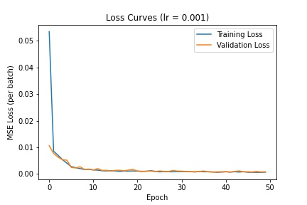
Training the model on a batch size of 128 with a learning rate of 1e-3 for 50 epochs produces the following loss curves.
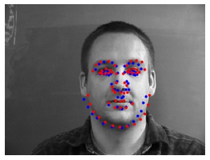
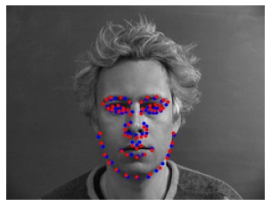
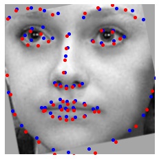
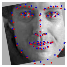
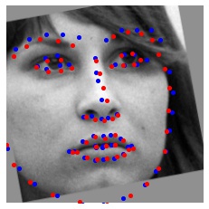
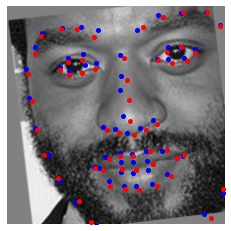
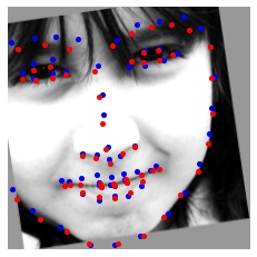
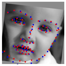
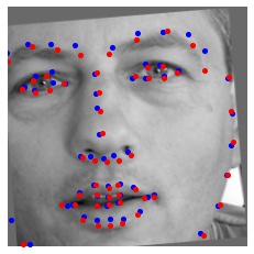
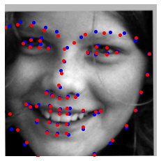
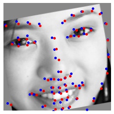
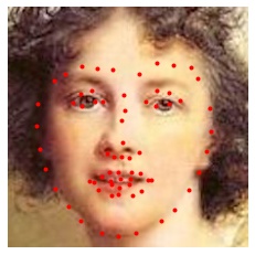
Here are the results; we compare the model's predictions (blue) with the ground-truth keypoints (red) for images in the validation dataset.
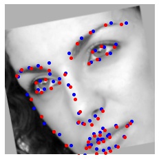
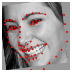
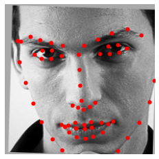
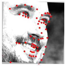
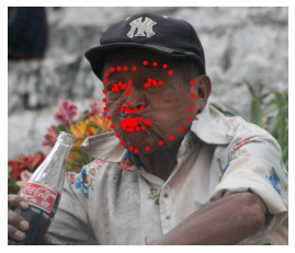
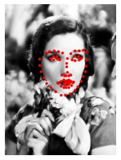
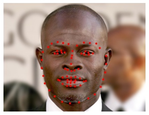
We can also predict facial keypoints on images in our Kaggle test dataset (which does not contain pre-annotated ground-truth facial keypoints). For the class Kaggle competition, my model scored a 7.87074. In the images below, the red points are the predicted keypoints.
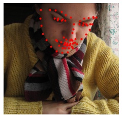
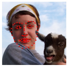
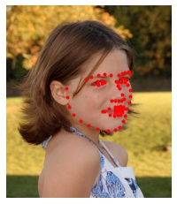
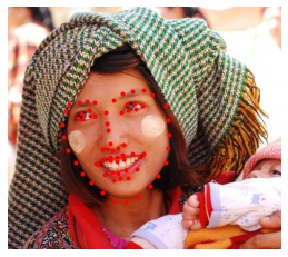
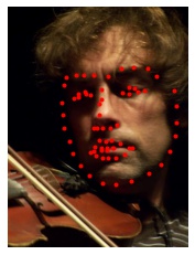
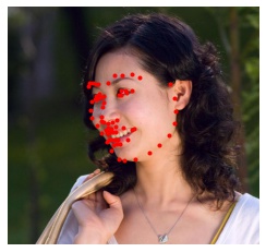

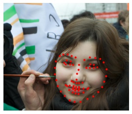
Finally, we can also predict facial keypoints on our own images. Here, I manually cropped the images to fit a 224x224 square before sending them to the CNN. Again, the red points are the predicted keypoints.
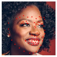
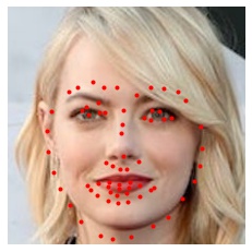
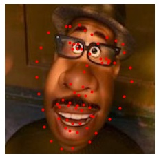
Since the CNN was trained on images where the face occupied a larger fraction of the image, the predictions here are not as good as those from the validation dataset. It's likely we will get better results if we had used the dlib facial detector to generate the bounding boxes for cropping because the model was trained on cropped images using this method. Not surprisingly, the model predicts keypoints better for realistic human faces than cartoon faces (e.g. Joe Gardner) which often have exaggerated facial proportions.