CS 194-26: Project 5

By Ana Cismaru

Part 1: Nose Tip Detection

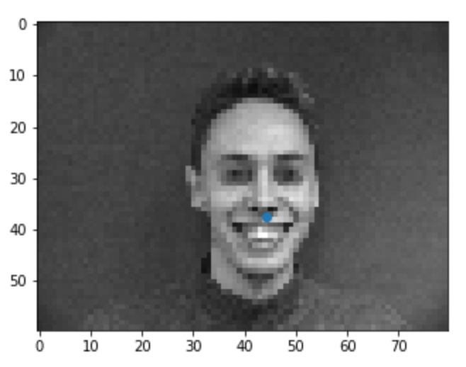
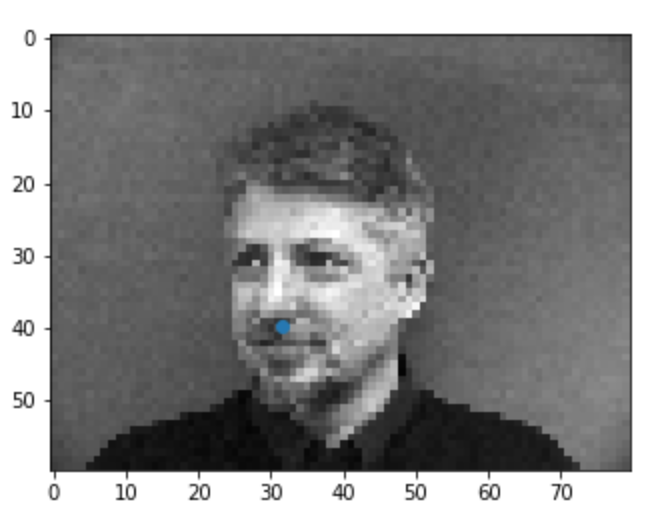
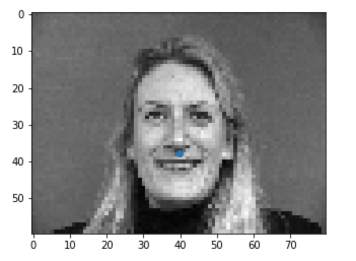
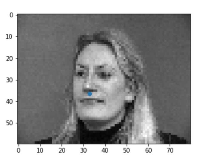
For the first part of this project, I set up a simple convolution network to locate the tip of the nose on an image of a person. The first thing we had to do is set up a dataloader and divide our data in a testing and training set. Below we can visualize this data.

Next, I set up a CNN model using the architecture below. This architecture was developed through some trial error, initally I had thought that more convolutional layers would lead to better results but in fact only using 3 layers instead of 4 proved to be better. Aside from the model architecture, I also had to set up a loss and optimizer. For that, I used the mean-squared error loss (MSELoss) and Adam as an optimizer with a learning rate of 0.0001. I trained the model for 20 epochs.

While training the model, we can visulize its training and validation loss to ensure that it is indeed decreasing (ie: the model is learning its task correctly).

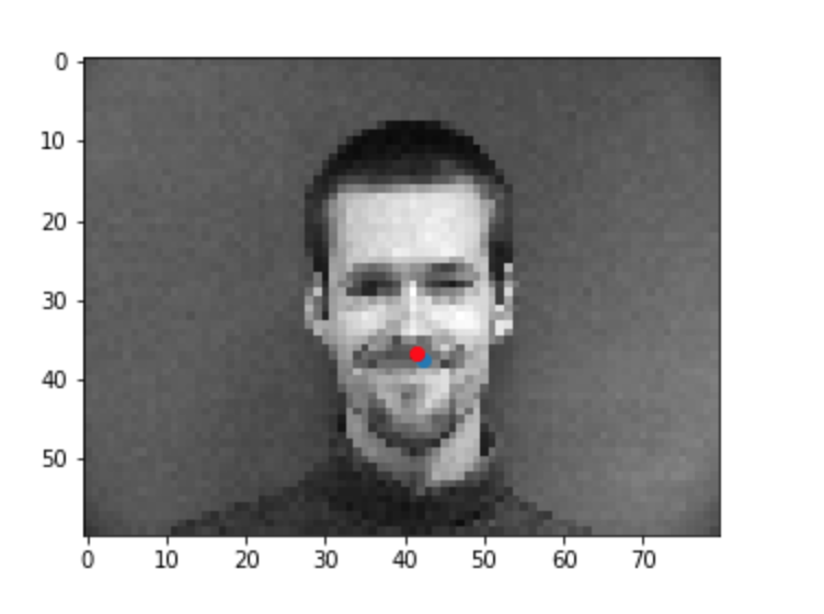
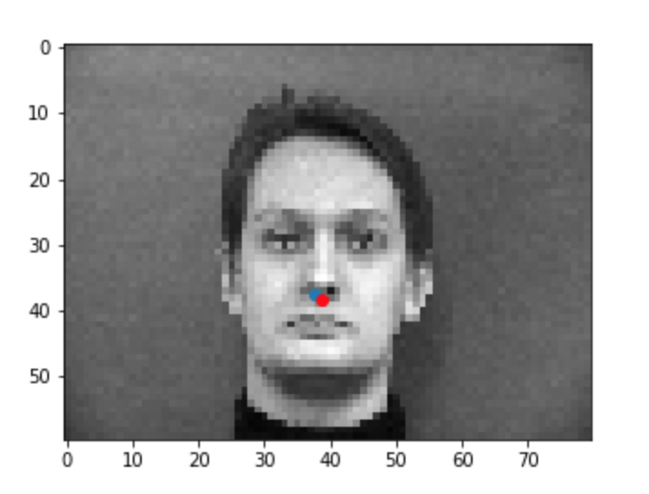
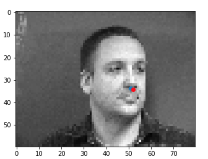
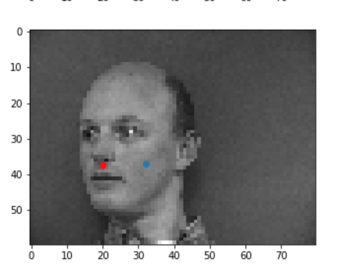
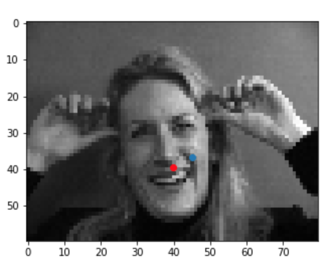
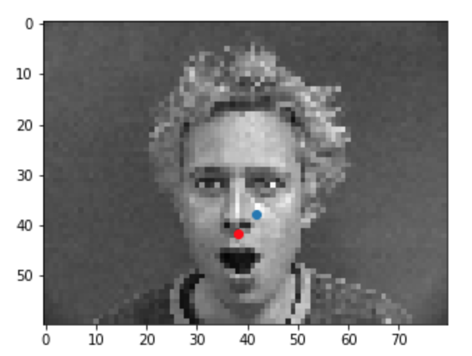
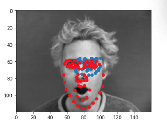
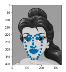
Once the model has trained, I ran it through a test set to visualize predictions on never before seen data. Below are some examples of the results with blue being my predictions and red being the ground truth. In certain instances such as when the person was facing straight forward, the model performed very well. In other cases such as when a person was facing at an angle or made funny expressions with their face, the model performed less well. This is probably due to the fact that the model learned facial features when people were making mostly serious faces and that those features were best visible at a straight angle (if the face was at an angle maybe some of the facial features were hidden/obscured or made more pronounced which could have confused the model).

Part 2: Face Landmark Detection (Small Dataset)

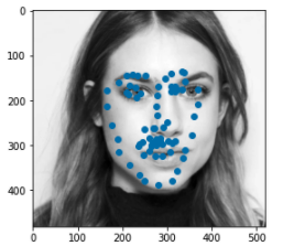
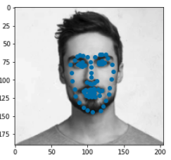
We'll now switch over to learning a more complicated task which is detecting all 58 facial landmarks from the Dane dataset. Similar to the first part, the first thing I did was set up a dataset and a dataloader. Since this was a more complicated task and we only had limited data. I also set up some data augmentations techniques to "create" more varied data for our model to learn off. The augmentations I used were horizontal and vertical flips (w/ p=0.2), rotation about the center of the image using angles between -15 and 15 (p=0.5), and translation in the x and y direction by [-10, 10] pixels (p=0.8). On top of that, I also performed a Color Jitter transformation (brightness = 0.5, contrast=0.8, saturation=0.8) to change the color structure of the image prior to converting it to grayscale. Below are some examples of the training data.

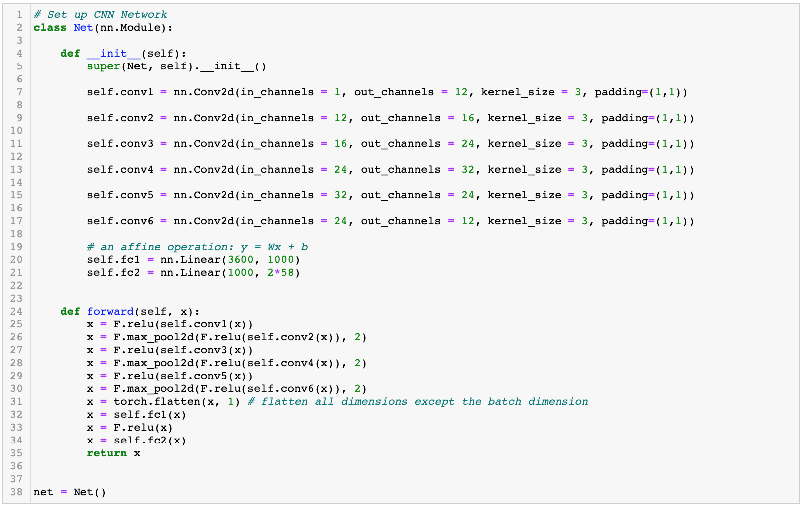
Next, we followed similar steps as before and set up the network. Below is the archecture that yielded the best results. Something interesting about this architecture is that we perform a maxpool at every other layer instead of at every layer. This improved results significantly which may be because more information is being passed on in those layers which is helping the model better learn the task.

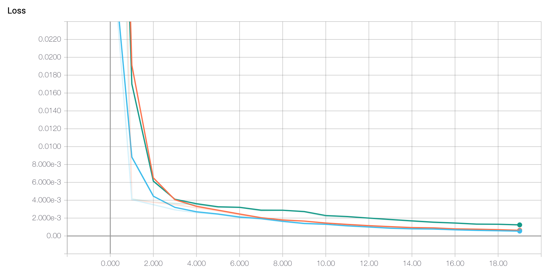
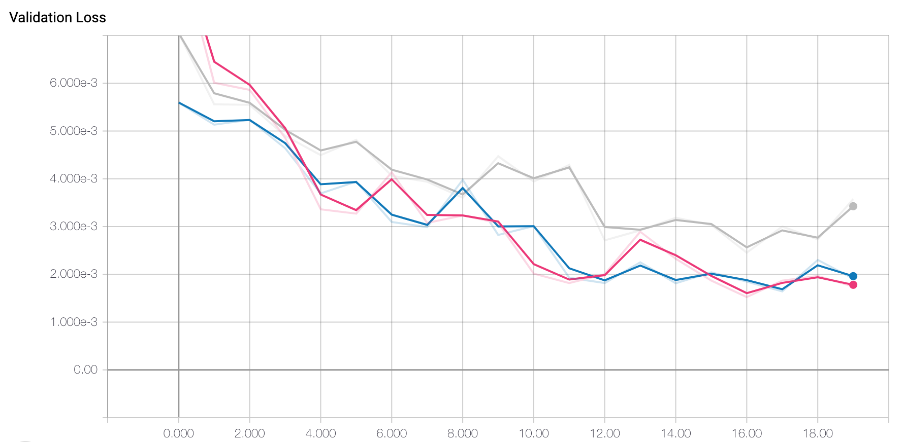
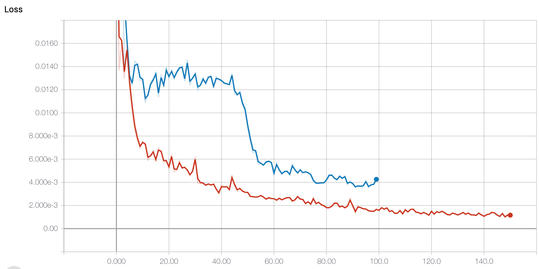
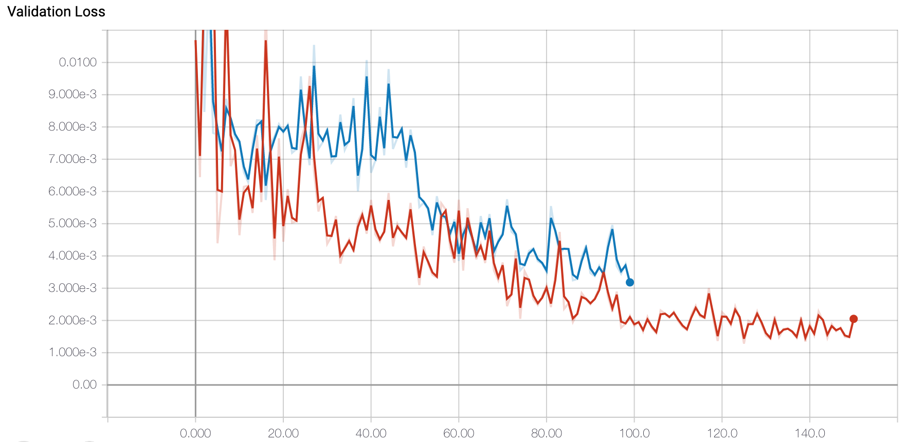
In terms of loss and optimzer, I again used MSE Loss and Adam optimizer with a learning rate of 0.0001. I then trained my best model for 150 epochs which is when it seemed to converge. In terms of hyperparameter tuning, I experimented with a batch size of 1 and a batch size of 16. I found that again the batch size of 1 seemed to work best. Below are the training and validation loss graphs.

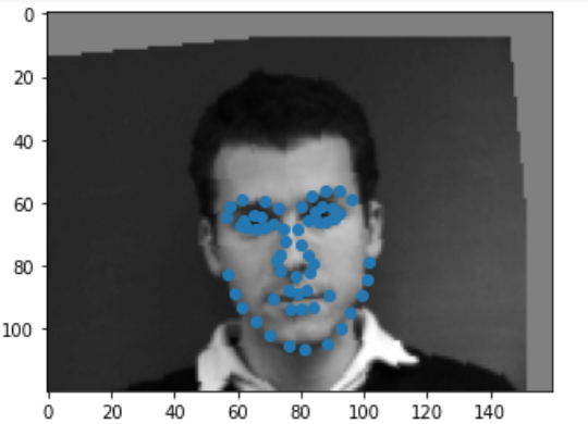
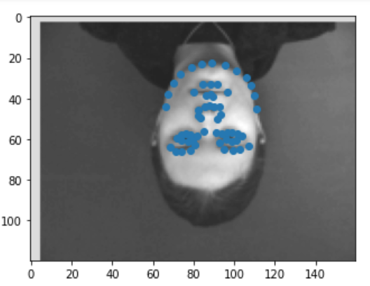
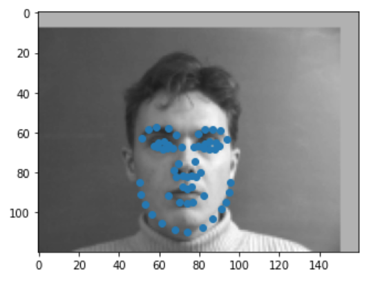
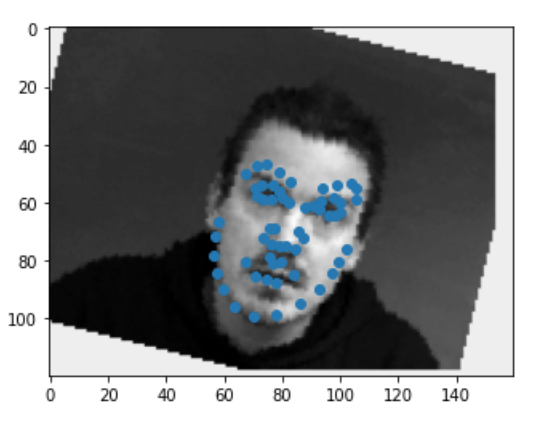
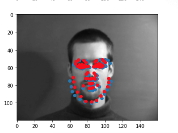
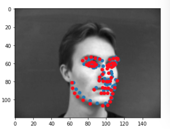
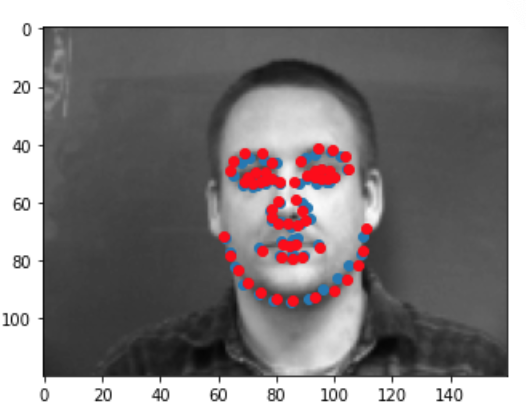
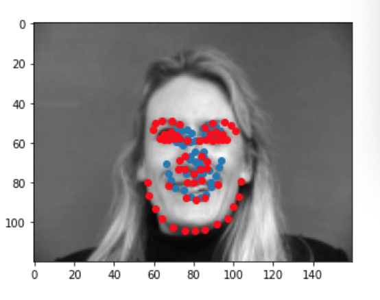
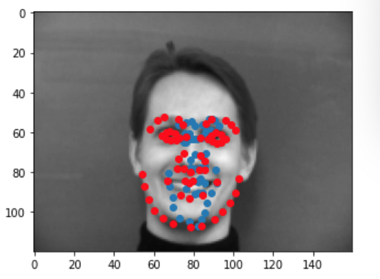
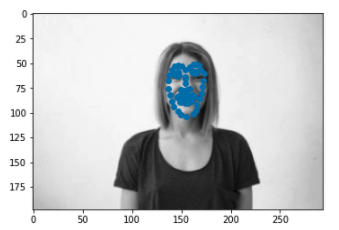
We can run our test dataset through the final model to visualize its predictions. Below are a couple examples of good prediction and bad predictions. Again, we notice that the model works best for male faces that have a serious expression, a sharp face, and minimal hair. This probably due to the fact that the majority of this dataset consists of this type of face. When we have deviations from this type of face ie: people with long hair, people with spiky, smiling person, yawning person... the model performs worse since it is not used to that type of face and may be confused by some of the other features (hair, smile lines, etc). Just like before, my predictions are in blue while the ground truth is in red.

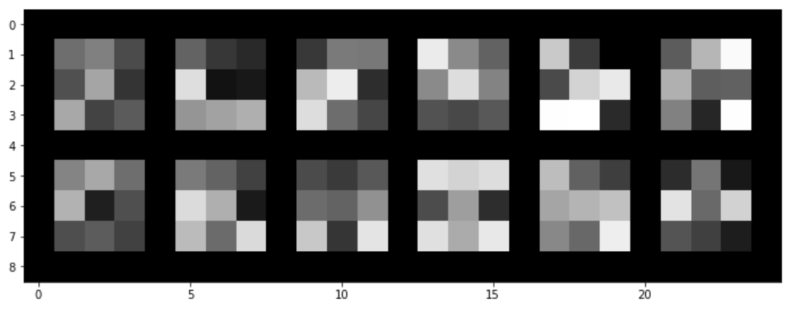
Another cool thing we can visualize about this model is its learned filters from the first layer. We can kind of see how some of the filters represent lines/edges, however they are not as clear as I had hoped.

Part 3: Train With Larger Dataset

The last part of this project consisted of using preexisting architectures to train a model on a large dataset to detect facial landmarks. The dataset consisted of images with faces in them, associated bounding boxes for the faces, and facial landmarks. The first thing I did was to preprocess the data to expand the bounding boxes by 150 pixels in the x and y direction since a lot of the boxes would crop of some of the landmarks. I also tried another experiment where I expanded the bounding boxes by 15% of the image size but that worked less effectively than expanding by 150 pixels. After that I filtered the data to only include images whose landmarks fall in the new bounding boxes (as some landmarks would also be out of the new larger bounding boxes). This resulted in using only 5034 images instead of 6666.

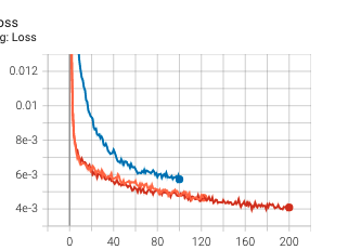
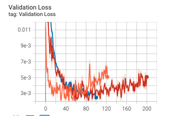
In terms of model architecture, I used a resnet18 model pretrained on ImageNet where I removed the last layer of the network and inserted a final layer that matches the landmark output. As an input to the model, I chose not to edit that first layer and instead simply stack the grayscale image 3 times before passing in as an input. With regards to datatloading, I chose a batch size of 32. With regards to the loss and optimizer, I again chose to use MSE and Adam. I experimented with a learning rate of of 1e-4 and 1e-5 and found that the former worked best. Below are images of the loss and validation loss for the three experiments I ran. One interesting thing we notice is that the validation loss ends up increasing for the red and orange experiment; that might be a sign that the model is beginning to overfit. I did try however running the model with an earlier epoch checkpoint but the results in terms of MAE on Kaggle were worse, so I'm not sure exactly what was happening for the loss to increase.

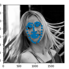
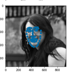
With regards to results, I score a 41.51 MAE on the Kaggle leaderboard. Some things I could have tried to further improve this result would be removing and retraining the first layer of the image, adding better preprocessing techniques to standardize face size even more, and maybe adding a scheduler to change the learning rate as the training progresses. Here are some examples of some good results and bad results from the training set.

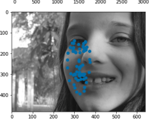
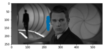
I also ran the algorithm on some photos of my choosing. One thing I noticed in my results is that the model works best on images where the face is far away (probably becuase we lose less resolution when resizing) so I tried running the model on some photos up close and photos far away to see if that claim stands for my data. I discovered that my model did work slightly better for faces that were far away but in general it worked alright. The points it seemed to struggle the most with were the chin outlines.