Facial Keypoint Detection with Neural Networks
Jeremy Warner — jeremy.warner at berkeley.edu
In this project, I learned how to use neural networks to automatically detect facial key points. For this project, I used PyTorch as the deep learning framework.
To start out, let’s build a network that just recognizes nose tips.
We will use the IMM face data set for this task (240 images).
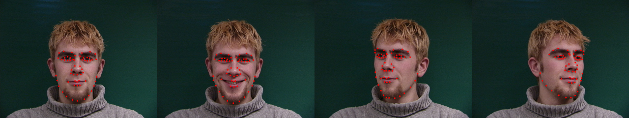
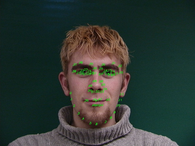
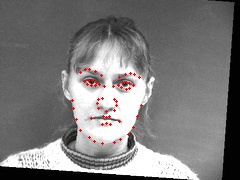
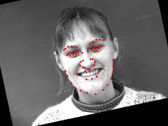
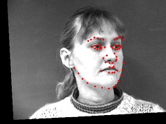
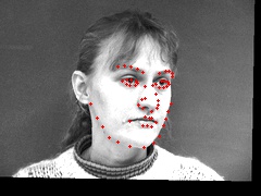
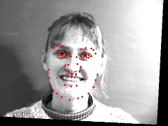
Viewing all of the points:
PIL seems to have the best algorithm for data retention when shrinking images.
image = image.resize(size, resample=PIL.Image.LANCZOS)Images after (80x60) resizing and normalization [-0.5, 0.5]:


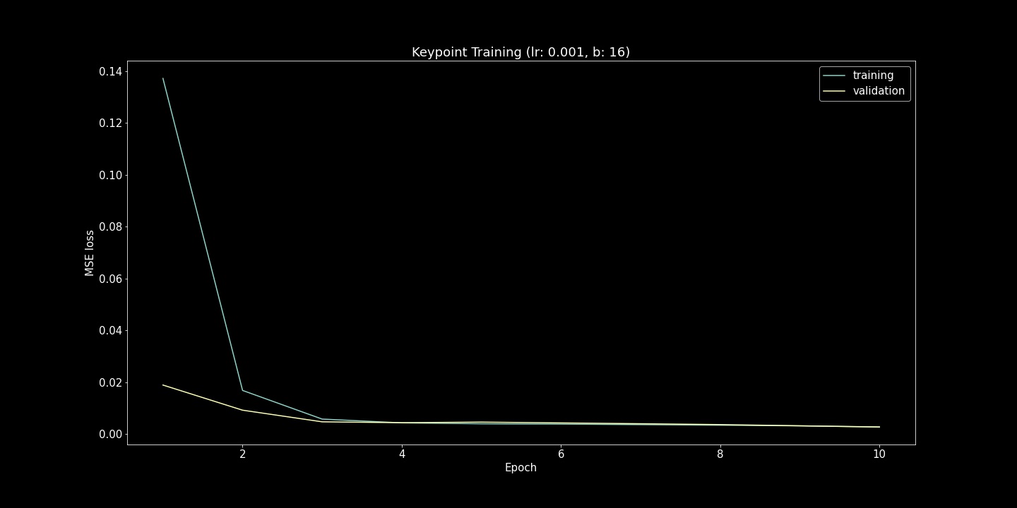
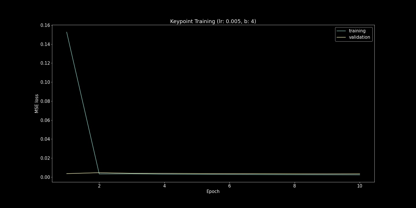
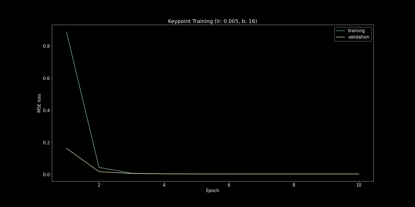
Using this network, I trained for 25 epochs and plot training and validation loss:
class Net(nn.Module):
    def __init__(self):
        super(Net, self).__init__()
        self.conv1 = nn.Conv2d(1, 32, 3, 1) # in, out, kernel, stride
        self.conv2 = nn.Conv2d(32, 32, 3, 1)
        self.conv3 = nn.Conv2d(32, 24, 3, 1)
        self.fc1 = nn.Linear(960, 128)
        self.fc2 = nn.Linear(128, 2)

    def forward(self, x):
        x = self.conv1(x)
        x = F.relu(x)
        x = F.max_pool2d(x, 2)
        x = self.conv2(x)
        x = F.relu(x)
        x = F.max_pool2d(x, 2)
        x = self.conv3(x)
        x = F.relu(x)
        x = F.max_pool2d(x, 2)
        x = torch.flatten(x, 1)
        x = self.fc1(x)
        x = F.relu(x)
        x = self.fc2(x)
        return x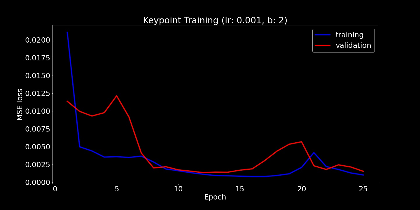
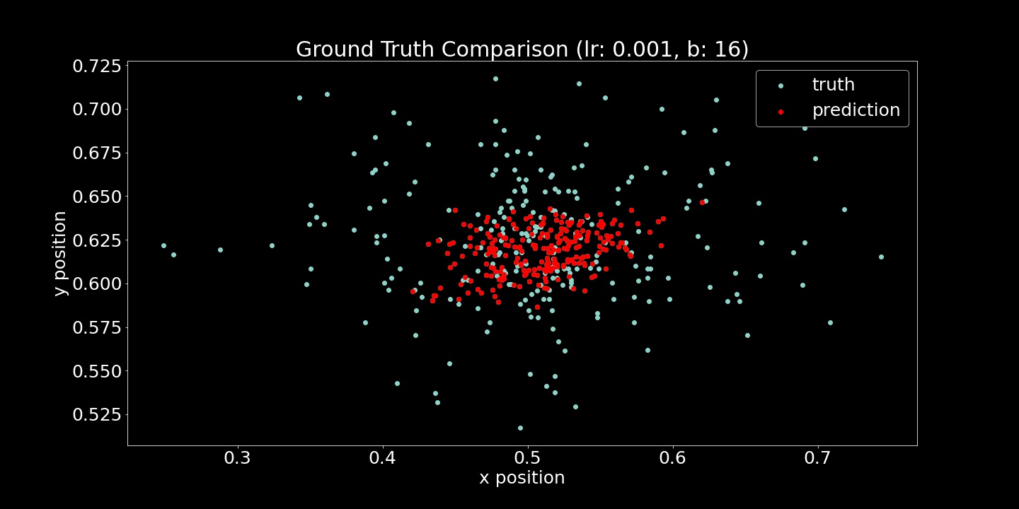
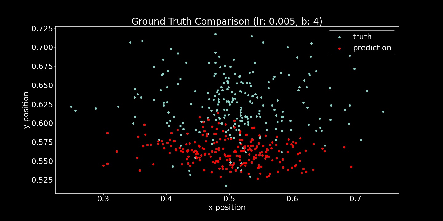
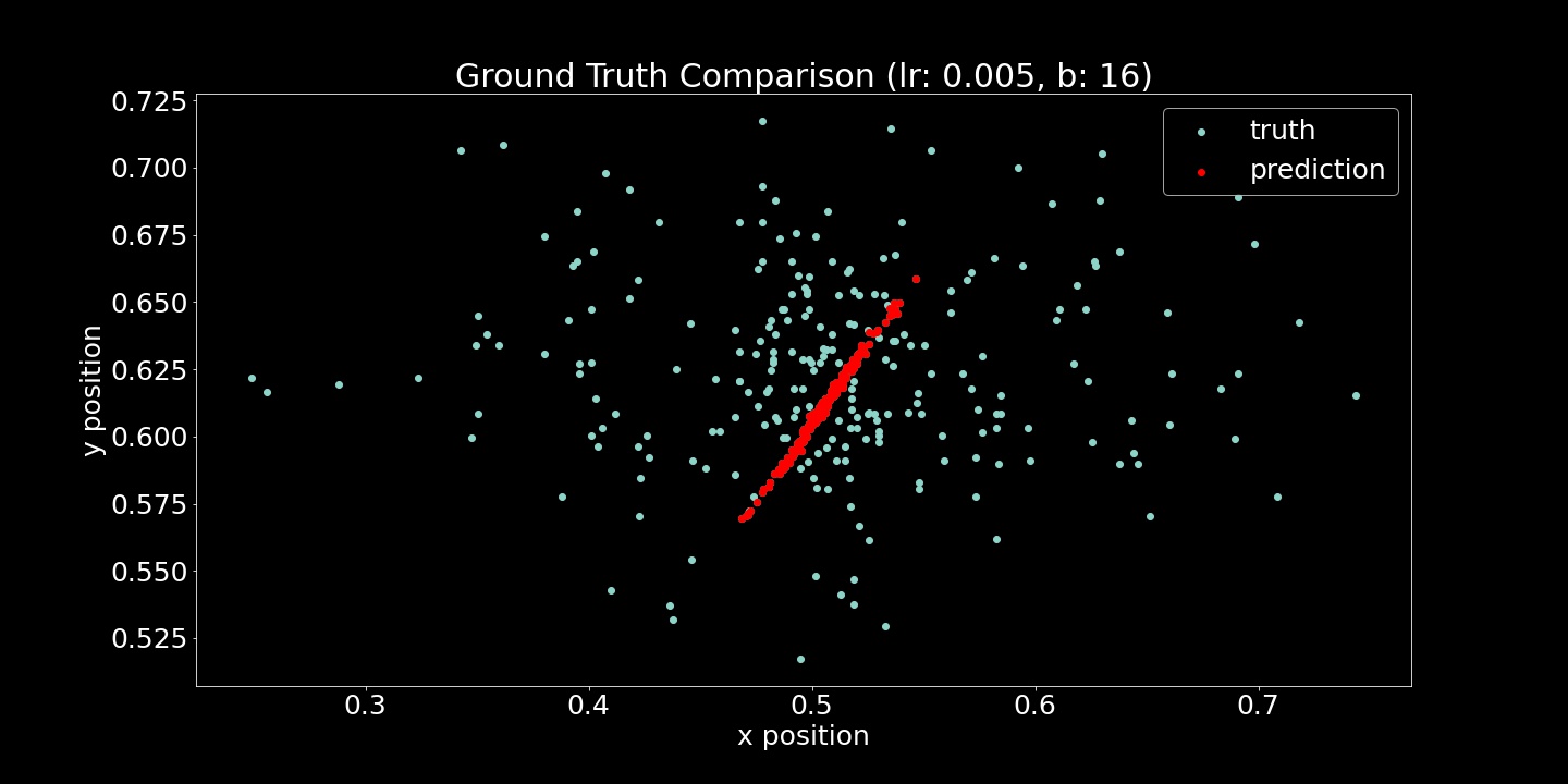
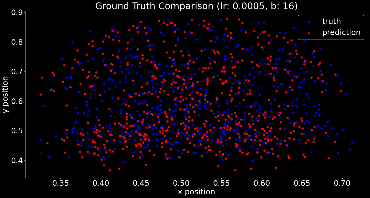
I show both the Mean Squared Error Loss (Training and Validation) and Ground Truth Comparison (scatter plots) here. For each of these hyperparameter comparisons, 10 epochs were run. While the loss function is useful to verify that the model is fitting to the provided examples, the scatter plots were also very useful. Seeing strange convergence artifacts like in the (lr=5e-5, b=16) example was surprising. Roughly gauging from these scatter plot examples, the learning rate effected the achieved accuracy more while batch size heavily influenced the density of model output range.
lr=1e-5, b=4
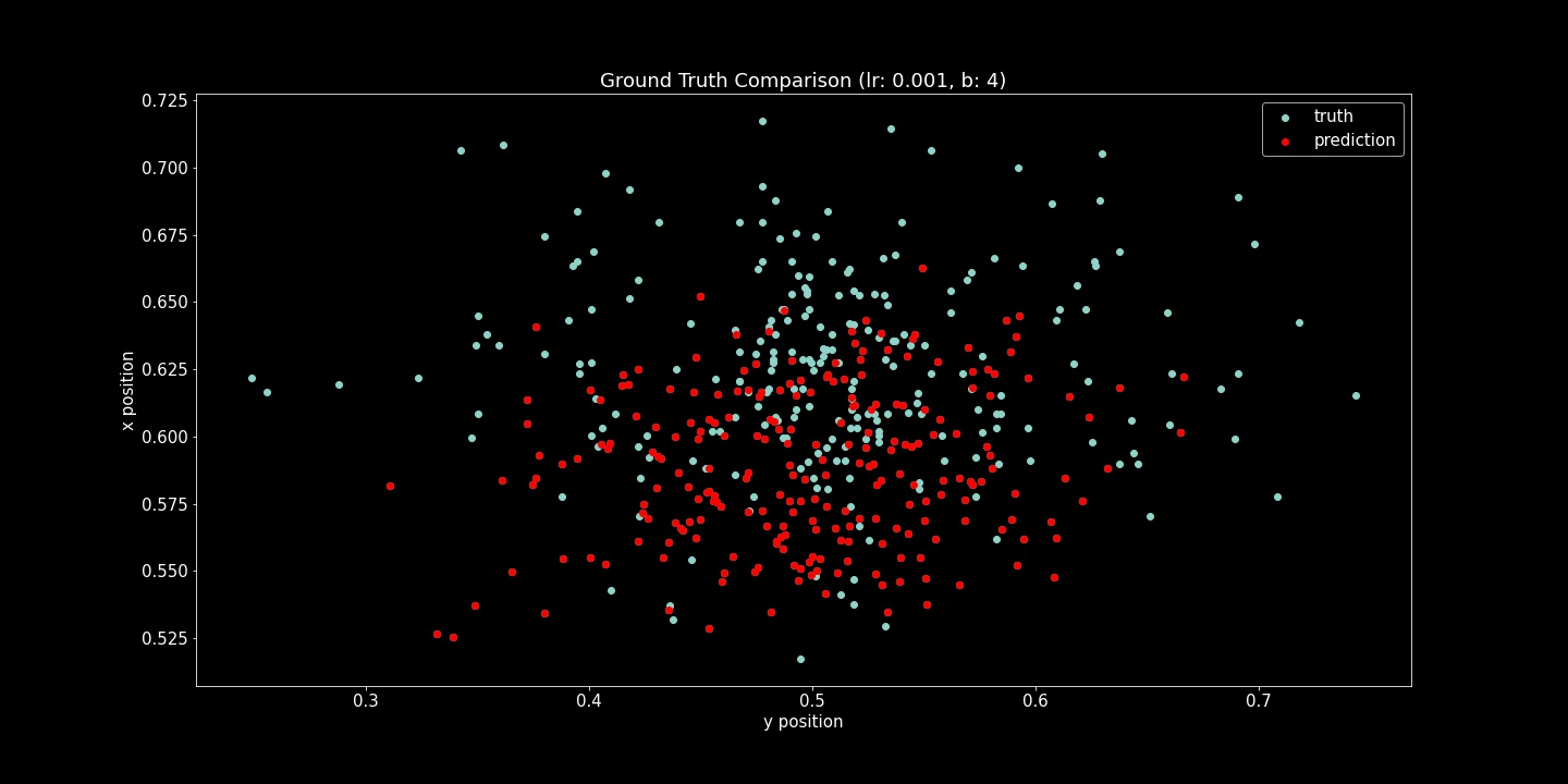
lr=1e-5, b=16
lr=5e-5, b=4
lr=5e-5, b=16
These image outputs were all creating with hyperparameters lr=1e-5, b=4.
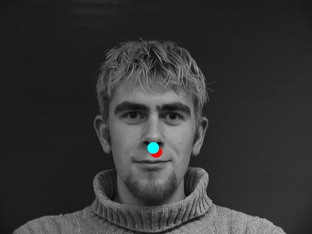
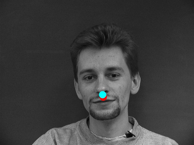
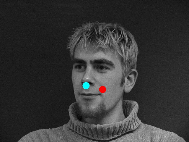
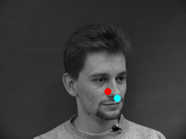
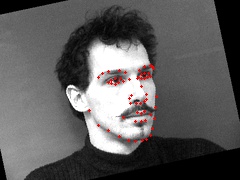
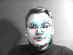
For the failure cases, both example faces are turned away from the camera. There are fewer examples to learn from where the face is turned like this. Thus, the model can learn less generally about the nose for these side angles. This is at least one interpretation of the performance difference.
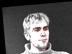
As the IMM data source only has 40 people (with 6 poses each), we need to augment the dataset to improve training. To do this, we can apply transformations to both the image and the key points used in training the network. I implemented data augmentation to the 240 image dataset, including ColorJitter (all 0.1), rotations (0-15 degrees), a 1/2 chance X-flip, and translation (5% image dimension). The dimensions of my augmented data and all key points:
Image: torch.Size([1, 180, 240])
Points: torch.Size([58, 2])
Here are more sampled images, overlaid with their transformed keypoints:

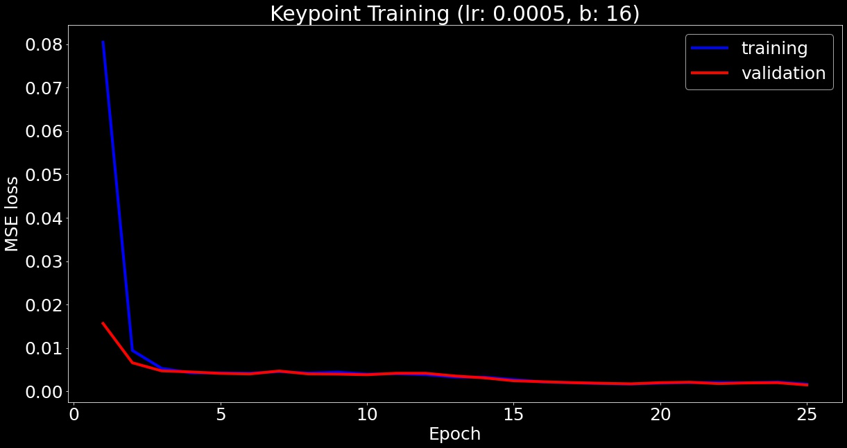
I bolstered the previous network with two additional convolutional layers. I reviewed the CS 231n CNN reference site and decided to keep the pooling layers the same. To account for the additional information from the new facepoints, I also increased channel width. When training, I ran for additional epochs, lowered the training rate to 5e-4, and increased batch to 16.
class Net(nn.Module):
    def __init__(self):
        super(Net, self).__init__()
        self.conv1 = nn.Conv2d(1,  32, 3, 1)
        self.conv2 = nn.Conv2d(32, 64, 3, 1)
        self.conv3 = nn.Conv2d(64, 64, 3, 1)
        self.conv4 = nn.Conv2d(64, 32, 3, 1)
        self.conv5 = nn.Conv2d(32, 24, 3, 1)
        self.fc1 = nn.Linear(12960, 1024)
        self.fc2 = nn.Linear(1024, 116)

    def forward(self, x):
        x = self.conv1(x)
        x = F.relu(x)
        x = self.conv2(x)
        x = F.relu(x)
        x = F.max_pool2d(x, 2)
        x = self.conv3(x)
        x = F.relu(x)
        x = self.conv4(x)
        x = F.relu(x)
        x = F.max_pool2d(x, 2)
        x = self.conv5(x)
        x = F.relu(x)
        x = F.max_pool2d(x, 2)
        x = torch.flatten(x, 1)
        x = self.fc1(x)
        x = F.relu(x)
        x = self.fc2(x)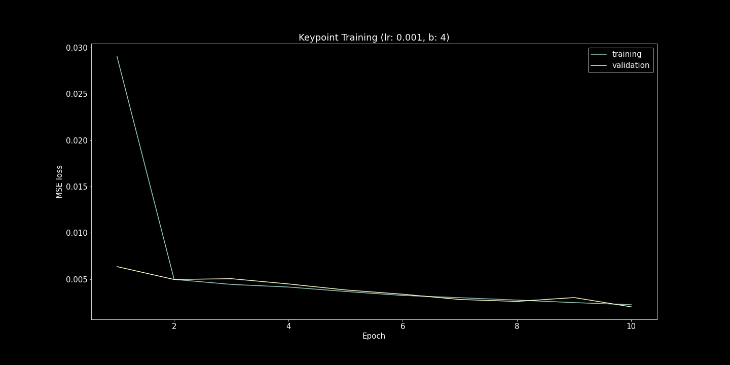
return xUsing this network, I trained for 25 epochs and plot training and validation loss:
Here is a scatter plot comparing predicted and truth keypoints:
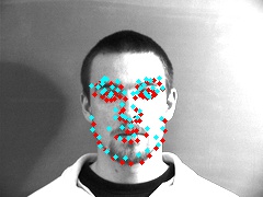
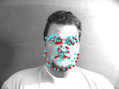
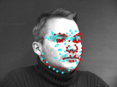
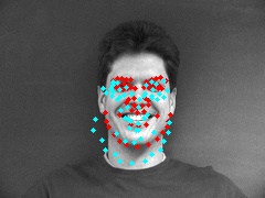
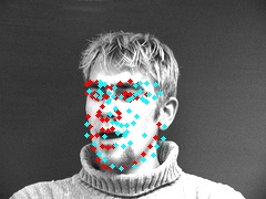
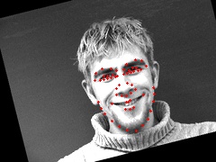
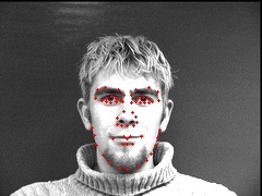
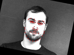
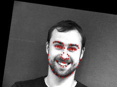
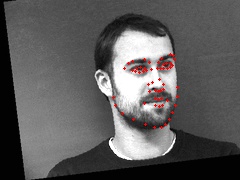
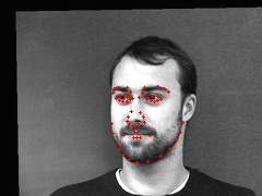
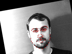
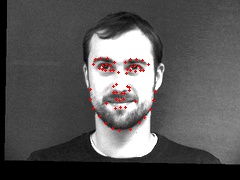
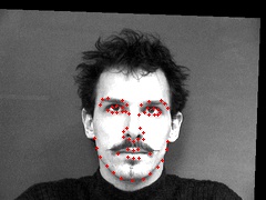
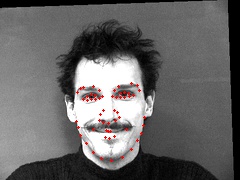
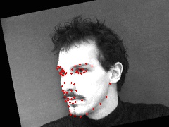
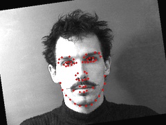
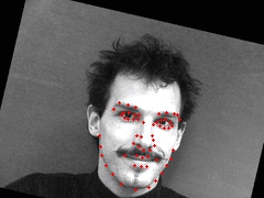
Qualitatively looking through the matches, I found that the network able to generate the most accurate keypoints for faces looking directly at the camera. The network started to learn about shifting face angles, but the majority of images were still looking straight forward. Additionally, the networks accuracy was greatly reduced on any image that had an open mouth or a smile.
Output of the first conv1 feature weights, after training as detailed above:
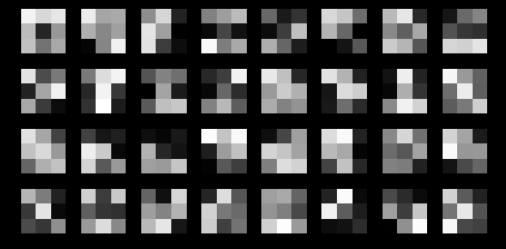
There are the basis of some edge detectors vaguely visible in the image.