Overview
In this project, I trained multiple neural networks to identify keypoints on face images.
Part 1: Nose Tip Detection
Dataloader
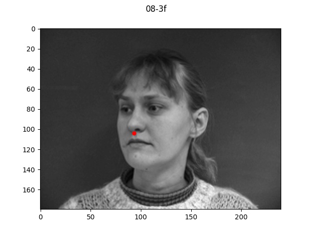
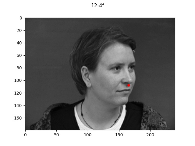
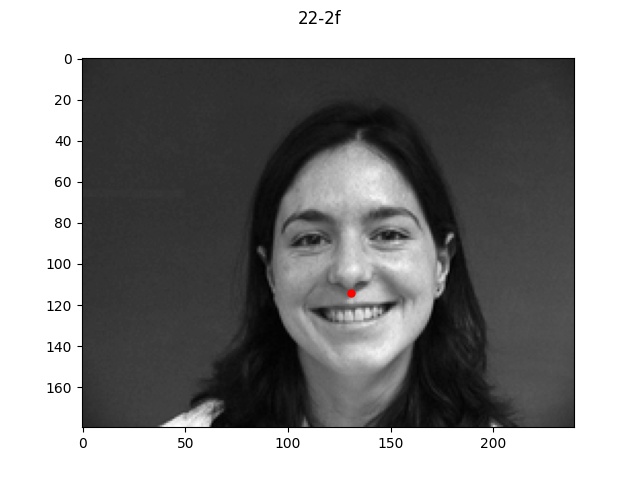
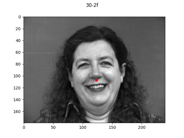
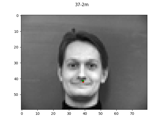
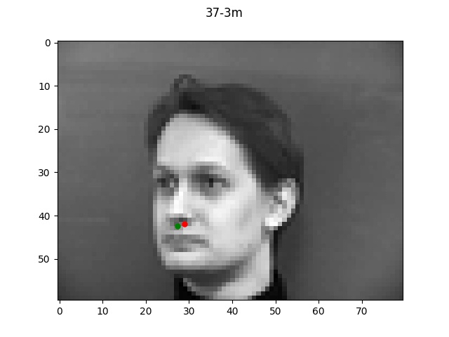
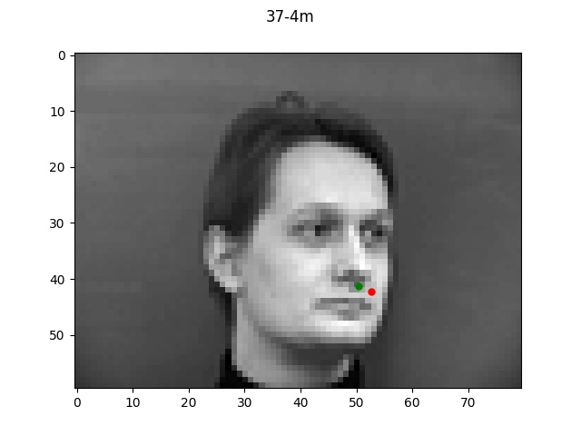
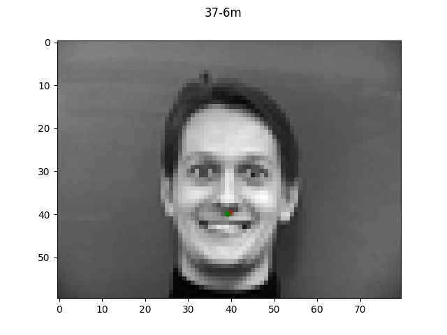
Here is a sample of four images and labeled keypoints that are loaded from my dataloader.
Network architecture
The architecture I used for nose detection consisted of the following layers:
- 12-channel Convolution layer with (7, 7) filter size
- ReLU
- MaxPool2d with window size 2
- 24-channel Convolution layer with (5, 5) filter size
- ReLU
- MaxPool2d with window size 2
- 32-channel Convolution layer with (3, 3) filter size
- ReLU
- MaxPool2d with window size 2
- Fully Connected Linear layer mapping input 896 dim to output 128 dim
- ReLU
- Fully Connected Linear layer mapping input 128 dim to output 2 dim
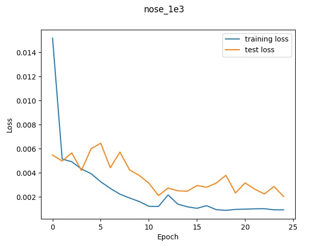
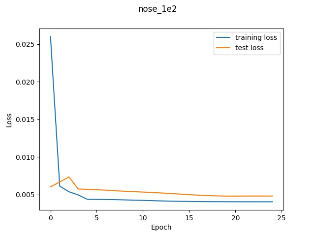
Performance
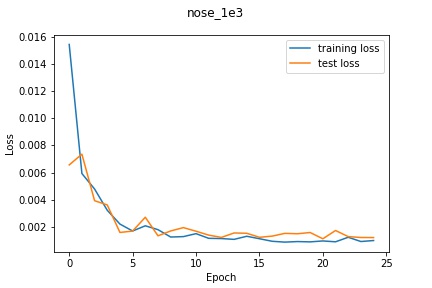
Using the default architecture described above with a learning rate of 1e-3, I noticed
decent performance. The loss graph and selected results are shown below.
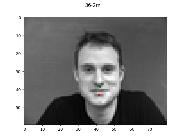
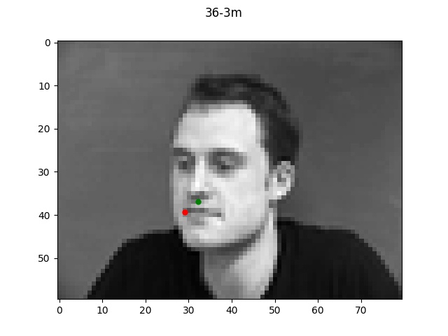
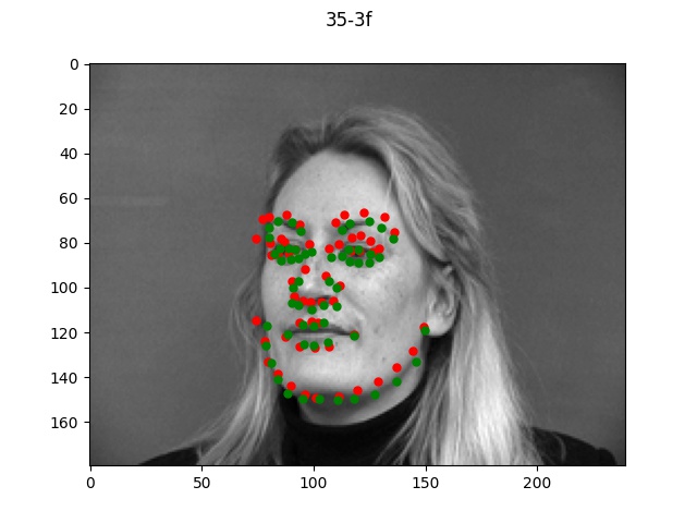
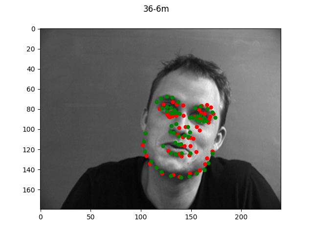
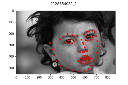
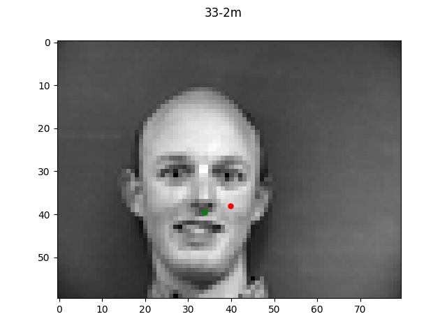
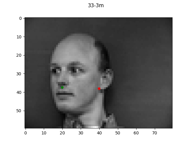
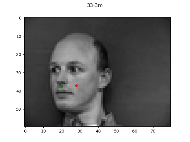
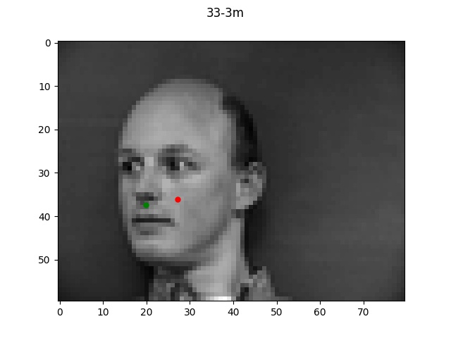
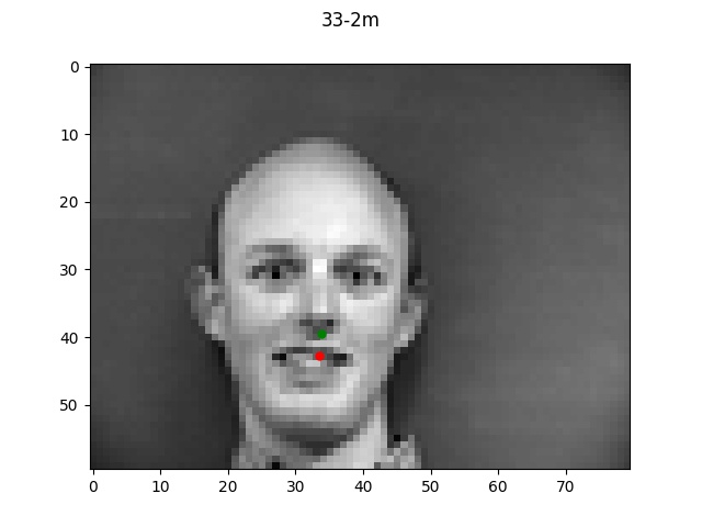
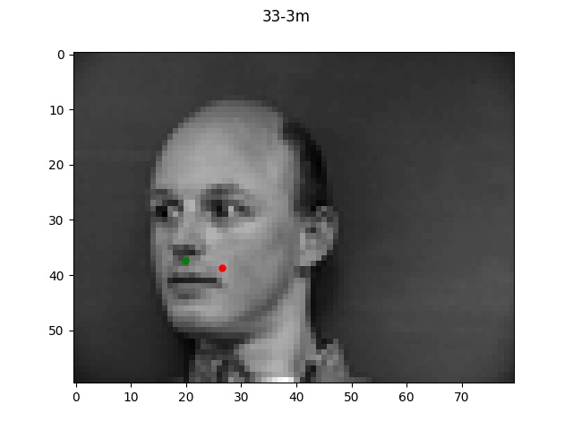
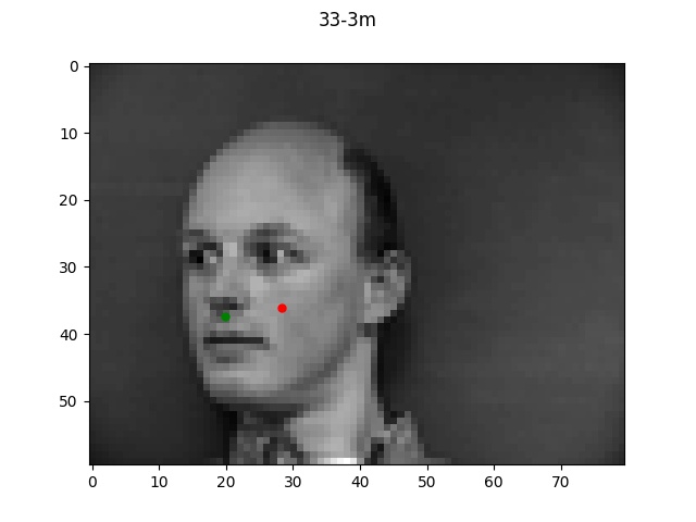
The green dot refers to the true point while the red dot is the predicted.
(Sorry, didn't realize they would be this small but if you zoom in, they should all be visible.)
Reflecting on the above examples, it seems like the model performed very well on the first face.
One reason for this might be that the first face looks a lot like the "average dane" face that
I created a couple projects ago. Since the face is very normal-looking in shape and expression, the
model did a much better job of learning it. The second face on the other hand has a longer chin
and a much more expressive mouth which is likely why the model got easily confused.
Different Learning Rates
The first hyperparameter I tried was using different learning rates. The results for 1e-2, 1e-3, and
1e-4 are shown below.
Loss Graphs
 Loss graph for 1e-2
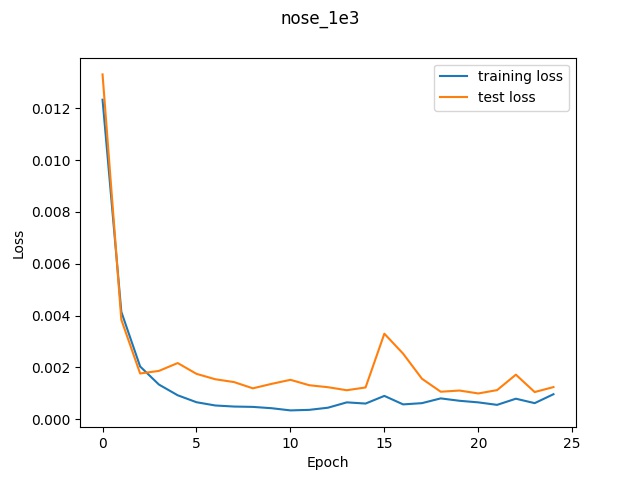 Loss graph for 1e-3
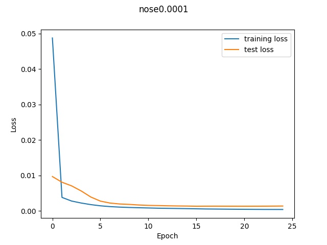 Loss graph for 1e-4
In the graphs, we can see that the higher learning rate (1e-2) had the worst validation
loss at well over 0.005 whereas the learning rate of 1e-3 was able to reach around 0.002
at the end and the learning rate 0f 1e-4 had a final validation loss of 0.0009. (This final
value is not obvious in the graph due to the poor axis labels but I printed out the loss at
each step and that's what it ended with). So according to the loss, it appears that the lower
learning ate performed the best.
Good example
 Detection for 1e-2
 Detection for 1e-3
 Detection for 1e-4
In these good examples, the 1e-2 learning rate performed a bit poorly but both the
two lower learning rates performed very well.
Bad example
 Detection for 1e-2
 Detection for 1e-3
 Detection for 1e-4
For the bad examples, the difference in learning rate is very obvious, with 1e-2 being pretty
far off while each decrease in learning rate brought the prediction point a bit closer to the true
label.
Different Filter Sizes
The second hyperparameter I tried was using different filter sizes for each conv layer. The results
for [(10,10), (7,7), (5,5)], [(7,7), (5,5), (3,3)] - default, and [(5,5), (3,3), (2,2)] are shown below.
Loss Graphs
 Loss graph for (5,5)
Loss graph for (7,7)
 Loss graph for (10,10)
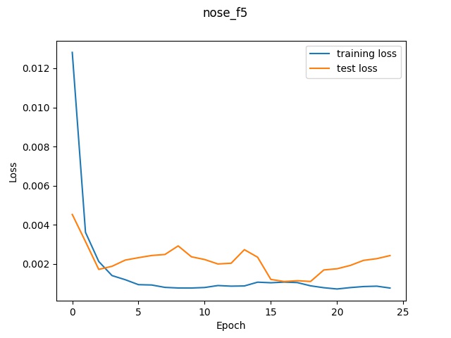
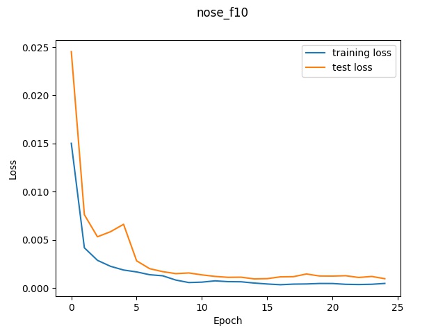
Looking at the graphs, it seems like the model with the largest filter sizes performed
relatively better since the smallest filter size had a very inconsistent validation
loss that was not strictly increasing whereas the largest filter size was a lot more stable
and increased lower to the lowest final loss.
Good example
 Detection for (5,5)
Detection for (7,7)
 Detection for (10,10)
In these good examples, the smallest filter size performed a bit poorly but both the
two higher filter sizes performed very well.
Bad example
 Detection for (5,5)
Detection for (7,7)
 Detection for (10,10)
For the bad examples, it actually seems like the lowest filter size performed a bit better
on this one since it's closer to the nose region; however, all of the models are still quite a bit off.
Part 2: Full Facial Keypoints Detection
Dataloader
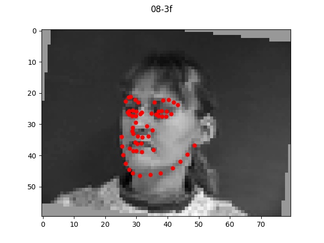
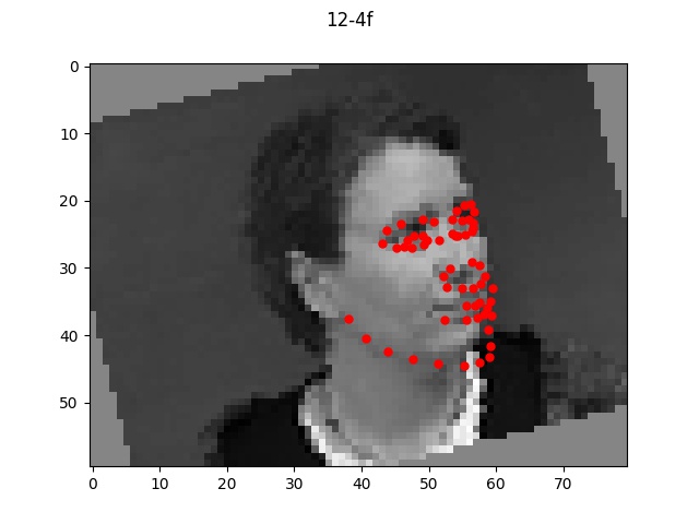
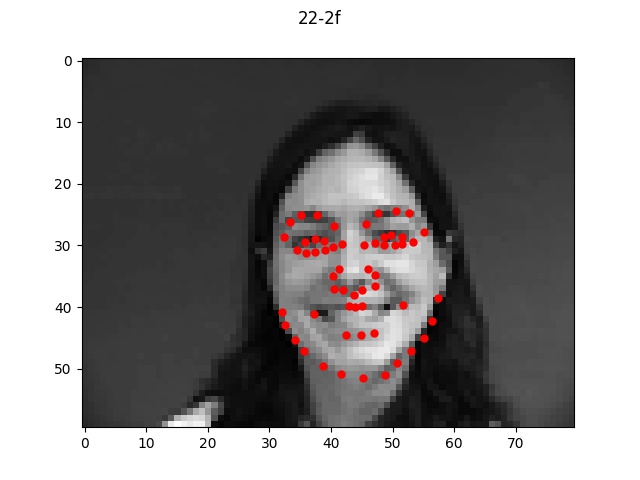
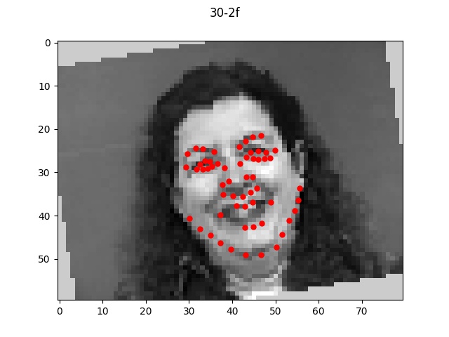
Here is a sample of four images and labeled keypoints that are loaded from my dataloader with random rotation augemntation.
Network architecture
The architecture I used for nose detection consisted of the following layers:
- 16-channel Convolution layer with (7, 7) filter size
- ReLU
- 32-channel Convolution layer with (7, 7) filter size
- ReLU
- 32-channel Convolution layer with (5, 5) filter size
- ReLU
- MaxPool2d with window size 2
- 64-channel Convolution layer with (5, 5) filter size
- ReLU
- MaxPool2d with window size 2
- 32-channel Convolution layer with (3, 3) filter size
- ReLU
- MaxPool2d with window size 2
- Fully Connected Linear layer mapping input 896 dim to output 128 dim
- ReLU
- Fully Connected Linear layer mapping input 128 dim to output 2 dim
The motiviation behind this architecture was to keep it simple and try to build off of
the architecture that had worked well for me with the nose detection. At first, I had tried
doing more max pool layers between convs and also having an additional conv layer; however, I found
that this network was too complicated and caused my model to predict the same types of
faces. Therefore, by removing some more layers, my model was able to perform significantly better.
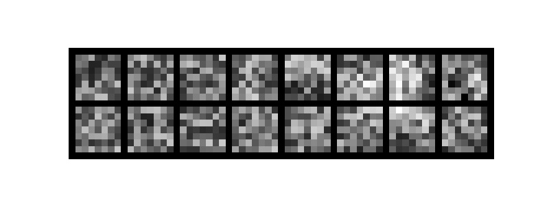
Convolution filters
Here are the 16 convolution filter weights from the first layer of my network. We can see that
each filter has a slightly different weight magnitude at each square which represents the different
feature types that each filter is learning.
Performance
Using the default architecture described above with a learning rate of 1e-3, I noticed
decent performance overall. The loss graph and selected results are shown below.
Sorry, forgot to update the title of the graph but it should be face_1e3.
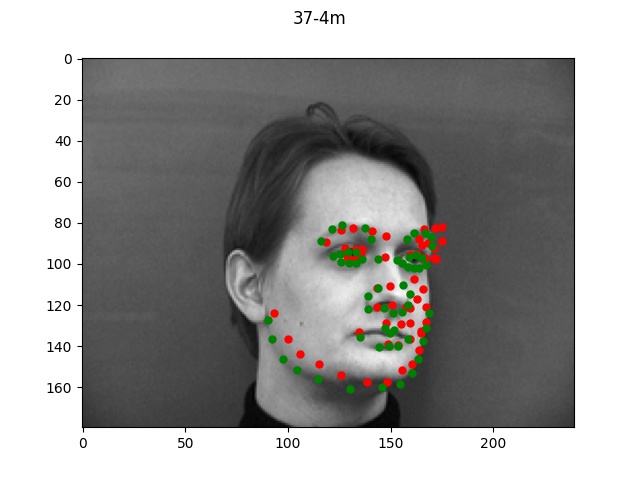
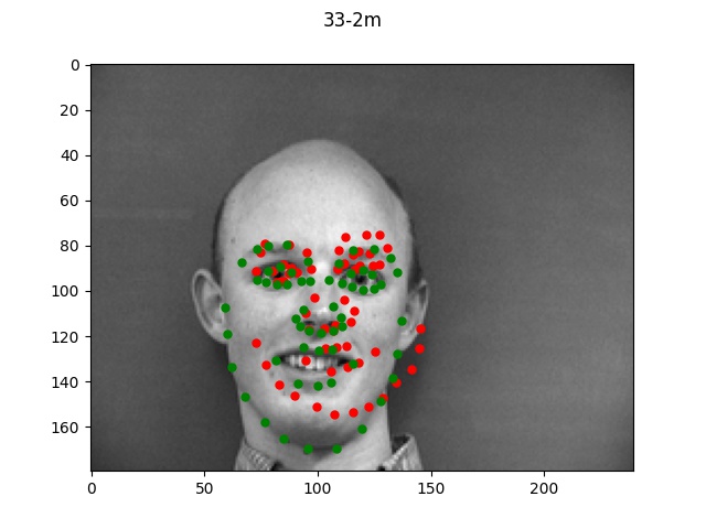
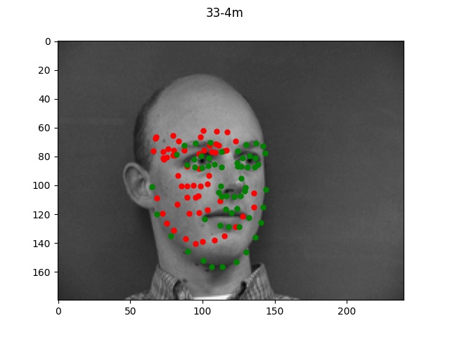
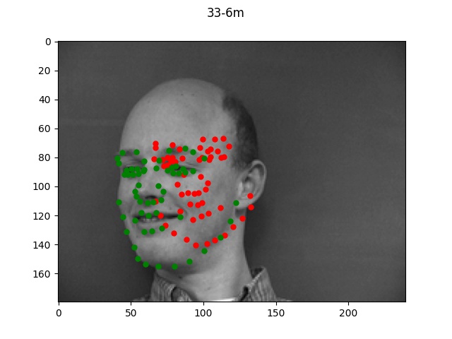
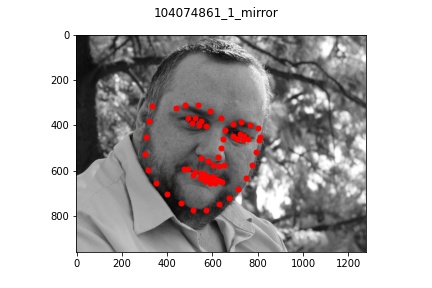
The green dots refers to the true points while the red dots is the predicted.
Looking at the good vs bad keypoints, it appears that the model for the most part performed
well when there was a clearly defined face with hair and facial features. The model performed
particularly poorly on male 33; this was likely due to the fact that this person was bald (lacking
hair which helped provide edge boundaries) and also his angled face is a lot more angled so these
two things together made it very difficult for the model to find the appropriate points.
Part 3: Train With Larger Dataset
Dataloader
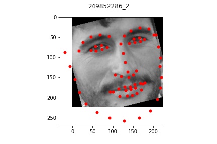
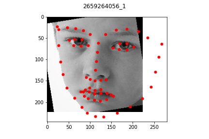
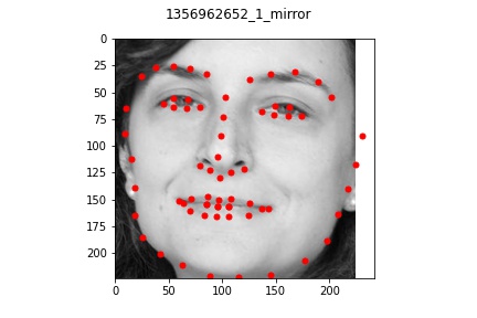
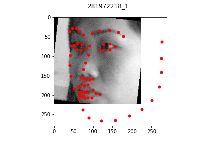
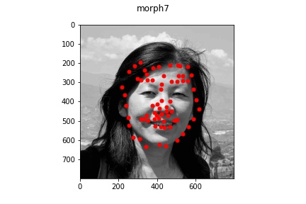
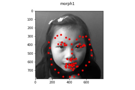
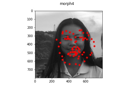
Here is a sample of four images and labeled keypoints that are loaded from my dataloader with random rotation augemntation.
Network architecture
The architecture I used for nose detection was a Resnet18 model with a modified first and final
layer to take in a black/white image and output 58 detected points:
            (conv1): Conv2d(1, 64, kernel_size=(7, 7), stride=(2, 2), padding=(3, 3), bias=False)

            (bn1): BatchNorm2d(64, eps=1e-05, momentum=0.1, affine=True, track_running_stats=True)

            (relu): ReLU(inplace=True)

            (maxpool): MaxPool2d(kernel_size=3, stride=2, padding=1, dilation=1, ceil_mode=False)

            (layer1): Sequential(

             (0): BasicBlock(

              (conv1): Conv2d(64, 64, kernel_size=(3, 3), stride=(1, 1), padding=(1, 1), bias=False)

              (bn1): BatchNorm2d(64, eps=1e-05, momentum=0.1, affine=True, track_running_stats=True)

              (relu): ReLU(inplace=True)

              (conv2): Conv2d(64, 64, kernel_size=(3, 3), stride=(1, 1), padding=(1, 1), bias=False)

              (bn2): BatchNorm2d(64, eps=1e-05, momentum=0.1, affine=True, track_running_stats=True)

             )

             (1): BasicBlock(

              (conv1): Conv2d(64, 64, kernel_size=(3, 3), stride=(1, 1), padding=(1, 1), bias=False)

              (bn1): BatchNorm2d(64, eps=1e-05, momentum=0.1, affine=True, track_running_stats=True)

              (relu): ReLU(inplace=True)

              (conv2): Conv2d(64, 64, kernel_size=(3, 3), stride=(1, 1), padding=(1, 1), bias=False)

              (bn2): BatchNorm2d(64, eps=1e-05, momentum=0.1, affine=True, track_running_stats=True)

             )

            )

            (layer2): Sequential(

             (0): BasicBlock(

              (conv1): Conv2d(64, 128, kernel_size=(3, 3), stride=(2, 2), padding=(1, 1), bias=False)

              (bn1): BatchNorm2d(128, eps=1e-05, momentum=0.1, affine=True, track_running_stats=True)

              (relu): ReLU(inplace=True)

              (conv2): Conv2d(128, 128, kernel_size=(3, 3), stride=(1, 1), padding=(1, 1), bias=False)

              (bn2): BatchNorm2d(128, eps=1e-05, momentum=0.1, affine=True, track_running_stats=True)

              (downsample): Sequential(

               (0): Conv2d(64, 128, kernel_size=(1, 1), stride=(2, 2), bias=False)

               (1): BatchNorm2d(128, eps=1e-05, momentum=0.1, affine=True, track_running_stats=True)

              )

             )

             (1): BasicBlock(

              (conv1): Conv2d(128, 128, kernel_size=(3, 3), stride=(1, 1), padding=(1, 1), bias=False)

              (bn1): BatchNorm2d(128, eps=1e-05, momentum=0.1, affine=True, track_running_stats=True)

              (relu): ReLU(inplace=True)

              (conv2): Conv2d(128, 128, kernel_size=(3, 3), stride=(1, 1), padding=(1, 1), bias=False)

              (bn2): BatchNorm2d(128, eps=1e-05, momentum=0.1, affine=True, track_running_stats=True)

             )

            )

            (layer3): Sequential(

             (0): BasicBlock(

              (conv1): Conv2d(128, 256, kernel_size=(3, 3), stride=(2, 2), padding=(1, 1), bias=False)

              (bn1): BatchNorm2d(256, eps=1e-05, momentum=0.1, affine=True, track_running_stats=True)

              (relu): ReLU(inplace=True)

              (conv2): Conv2d(256, 256, kernel_size=(3, 3), stride=(1, 1), padding=(1, 1), bias=False)

              (bn2): BatchNorm2d(256, eps=1e-05, momentum=0.1, affine=True, track_running_stats=True)

              (downsample): Sequential(

               (0): Conv2d(128, 256, kernel_size=(1, 1), stride=(2, 2), bias=False)

               (1): BatchNorm2d(256, eps=1e-05, momentum=0.1, affine=True, track_running_stats=True)

              )

             )

             (1): BasicBlock(

              (conv1): Conv2d(256, 256, kernel_size=(3, 3), stride=(1, 1), padding=(1, 1), bias=False)

              (bn1): BatchNorm2d(256, eps=1e-05, momentum=0.1, affine=True, track_running_stats=True)

              (relu): ReLU(inplace=True)

              (conv2): Conv2d(256, 256, kernel_size=(3, 3), stride=(1, 1), padding=(1, 1), bias=False)

              (bn2): BatchNorm2d(256, eps=1e-05, momentum=0.1, affine=True, track_running_stats=True)

             )

            )

            (layer4): Sequential(

             (0): BasicBlock(

              (conv1): Conv2d(256, 512, kernel_size=(3, 3), stride=(2, 2), padding=(1, 1), bias=False)

              (bn1): BatchNorm2d(512, eps=1e-05, momentum=0.1, affine=True, track_running_stats=True)

              (relu): ReLU(inplace=True)

              (conv2): Conv2d(512, 512, kernel_size=(3, 3), stride=(1, 1), padding=(1, 1), bias=False)

              (bn2): BatchNorm2d(512, eps=1e-05, momentum=0.1, affine=True, track_running_stats=True)

              (downsample): Sequential(

               (0): Conv2d(256, 512, kernel_size=(1, 1), stride=(2, 2), bias=False)

               (1): BatchNorm2d(512, eps=1e-05, momentum=0.1, affine=True, track_running_stats=True)

              )

             )

             (1): BasicBlock(

              (conv1): Conv2d(512, 512, kernel_size=(3, 3), stride=(1, 1), padding=(1, 1), bias=False)

              (bn1): BatchNorm2d(512, eps=1e-05, momentum=0.1, affine=True, track_running_stats=True)

              (relu): ReLU(inplace=True)

              (conv2): Conv2d(512, 512, kernel_size=(3, 3), stride=(1, 1), padding=(1, 1), bias=False)

              (bn2): BatchNorm2d(512, eps=1e-05, momentum=0.1, affine=True, track_running_stats=True)

             )

            )

            (avgpool): AdaptiveAvgPool2d(output_size=(1, 1))

            (fc): Linear(in_features=512, out_features=136, bias=True)
I printed out the model's named children and copied it above to show the names of each layer in the model.
We can also see the dimensions of the model, where it is clear that I modified the input layer to take in a
dimension-1 image (since my inputs are black and white) and also changed the output to have 136 features which
represents a flattened 2-d array of 58 points.
Performance
Using the Resnet18 architecture described above with a learning rate of 1e-3, I scored
a 12.09849 mean absolute error (https://www.kaggle.com/aliu917). The loss graph from
training is shown below:
Sorry, forgot to update the title of the graph but it should be train_1e3.
Looking at the graph, the loss decrease shape looks very good with both train and validation loss
decreasing pretty in sync. It looks like the loss has mostly flattened out in the end but
perhaps training for longer may have seen the loss graph go even closer towards 0 since it
appears to still be on a slightly decreasing trend at the end of 25 epochs.
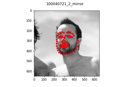
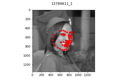
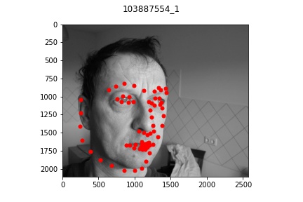
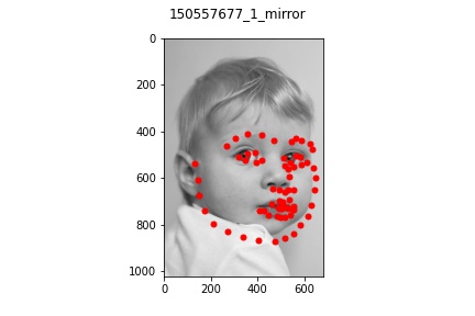
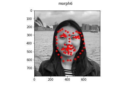
Overall, my model performed very well on most faces even of different orientations and I'm
quite impressed by the results that turned out. There were a few cases where the model
seemed to be a bt off from the actual face which I pictured above. In each bad example case,
the faces all exhibit a slightly unusual shape or angle (first one is very angled with hair,
second one has a very long face, and third one is very light/pale colored with a very round face shape).
Part 3: Training on my own Data
It appears that for the most part, the model did okay on my own data but did perform
noticeably worse than on the actual train/test set data provided. This is lkely due to
multiple reasons: some of the older pictures (those in the bad example) have a lot
lower resolution which makes the image a bit blurrier and likely contributed to the
model's difficulty in learning and identifying facial features. Another reason might be that
my bounding boxes (which I estimated myself) were not as accurate which resulted in
poor predictions. But overall, the model was able to recognize some of the face features at least!