Project 5: Facial Keypoint Detection with Neural Networks - Joe Zou
Part 1: Nose Tip Detection
1.1 Samples from DataLoader
For this part, I implemented a DataLoader with three transforms that convert the image to grayscale, normalizes the pixel values to be between -0.5 and 0.5, and resizes the image to 80x60. Here are some samples taken from the data loader:
.png)
.png)
.png)
1.2 Hyper Parameter Tuning and Loss Plots
My model has 4 conv layers followed by 2 fc layers. The 4 conv layers are all followed by a ReLU and maxpool while the first fc layer is followed by a ReLU. I performed hyper parameter tuning on batch size, learning rate, convolution filter size, and convolutional channel widths. I've included some of the training and validation loss plots below. The names of the models are written in the format {filter_size}_{conv channels}_{lr}_{bs}_{epochs}
3_(16,32,64,128)_0.001_32_20
.png)
5_(16, 32, 64, 128)_0.001_32_20
.png)
3_(16,32,64,128)_0.001_8_20
.png)
3_(16,32,64,128)_0.0003_8_20
.png)
3_(64,64,128,256)_0.0006_8_20
.png)
3_(64,128,256,512)_0.0006_8_50
.png)
5_(64, 128, 256, 256)_0.0006_8_50 [THE FINAL MODEL I USED]
.png)
1.3 Effect of Hyper Parameter Tuning
From my hyper parameter tuning experiments, we can see that increasing the convolution channels of the model from something like (16, 32, 64, 128) to (64, 128, 256, 256) allowed the training loss to get lower from 1.2e-4 to something like 1.5e-5. It also seems like decreasing the learning rate enabled the model to train to a lower loss. Finally, increasing the number of epochs for training helped the validation loss stabilize at a lower value which is best shown in the last two loss plots.
1.4 Success and Failure Cases
Success Cases
.png)
.png)
Failure Cases: These cases seem to have failed because the faces are turned to the side, so the model struggles more to find the nose.
.png)
.png)
Part 2: Full Facial Keypoints Detection
2.1 Samples from DataLoader
For this part, I added on two data augmentation techniques to the data loader from part 1. The first data augmentation is a rotation by sampled from a normal distribution centered around 0 with standard deviation of 7.5. The second data augmentation is a translation by each sampled from a normal distribution centered around 0 with standard deviation of 10. Here are some samples from the data loader:
.png)
.png)
.png)
2.2 Model Architecture

The final model architecture I decided on is:
input(1,180,240) → conv(128), relu, conv(128), relu, maxpool, conv(256), relu, conv(256), relu, maxpool, conv(256), relu, conv(256), relu, maxpool, fc(512), relu, fc(116) → output(116)
The convention I use is conv(out_channels) and fc(out_dims) as the in_channels and in_dims can both be calculated from the prior layers. The convolution filter_size I ended up using was 5.
There are essentially 3 repeated blocks of convolutions where each block consists of conv(channel), relu, conv(channel), relu, maxpool. The convolution channel dimensions stay constant within each block and the image dimension remains the same until it is halved by the maxpool at the end. Following these three repeated blocks of convolution operations is two fully connected layers separated by a ReLU activation. The exact dimensions of the convolution channels and filter_size were found from hyper parameter tuning explained below.
2.3 Hyper Parameter Tuning and Loss Plots
I performed hyper parameter tuning on batch size, learning rate, convolution filter size, and convolutional channel dimensions. I've included some of the training and validation loss plots below. The names of the models follow the same convention as part 1 of {filter_size}_{conv channels}_{lr}_{bs}_{epochs}. Note that these plots I've displayed are from the later half of my hyperparameter tuning. My colab notebook reset and lost some of the plots of a model with much smaller convolutional channels and filter sizes, but those models overall had worse training loss so those results are not too significant.
5_(128,256,512)_5e-5_8_50
.png)
5_(128,256,512)_0.0003_8_50
.png)
5_(128,256,512)_0.0006_8_50
.png)
5_(128,256,512)_0.0006_4_50
.png)
5_(128,256,256)_0.0003_4_75 [MODEL I DECIDED TO USE]
.png)
5_(64, 256, 256)_0.0006_4_75
.png)
2.4 Success and Failure Cases
I display some predictions the model makes on the validation set.
Success Cases:
.png)
.png)
Failure Cases: it seems like the model still struggles with strange expressions or turned faces
.png)
.png)
2.5 Visualizing Learned Features
I visualized the filters of the first convolutional layer for my final model. As I mentioned above in the model architecture details, the first convolutional layer has 128 output channels which is why there are 128 filters visualized here:
.png)
Part 3: Train with Larger Dataset
3.1 Kaggle Submission
I submitted my final model to the kaggle competition with a score(MAE) of 8.69294 on the public test set. My kaggle email is: joezou@berkeley.edu
3.2 Detailed Model Architecture
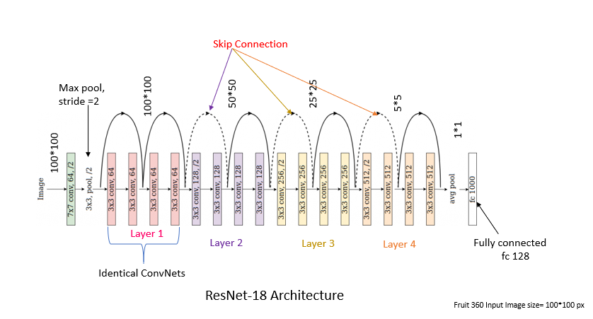
I've included the code snippet to create my model architecture along with the detailed architecture. The model i use is a pre-trained resnet18 with the input to the first convolution layer changed from 3→1 and the output of the last linear layer changed from 1000→136. I actually just replaced these blocks so these two layers will lose the pre-trained weights.

ResNet(
  (conv1): Conv2d(1, 64, kernel_size=(7, 7), stride=(2, 2), padding=(3, 3), bias=False)
  (bn1): BatchNorm2d(64, eps=1e-05, momentum=0.1, affine=True, track_running_stats=True)
  (relu): ReLU(inplace=True)
  (maxpool): MaxPool2d(kernel_size=3, stride=2, padding=1, dilation=1, ceil_mode=False)
  (layer1): Sequential(
    (0): BasicBlock(
      (conv1): Conv2d(64, 64, kernel_size=(3, 3), stride=(1, 1), padding=(1, 1), bias=False)
      (bn1): BatchNorm2d(64, eps=1e-05, momentum=0.1, affine=True, track_running_stats=True)
      (relu): ReLU(inplace=True)
      (conv2): Conv2d(64, 64, kernel_size=(3, 3), stride=(1, 1), padding=(1, 1), bias=False)
      (bn2): BatchNorm2d(64, eps=1e-05, momentum=0.1, affine=True, track_running_stats=True)
    )
    (1): BasicBlock(
      (conv1): Conv2d(64, 64, kernel_size=(3, 3), stride=(1, 1), padding=(1, 1), bias=False)
      (bn1): BatchNorm2d(64, eps=1e-05, momentum=0.1, affine=True, track_running_stats=True)
      (relu): ReLU(inplace=True)
      (conv2): Conv2d(64, 64, kernel_size=(3, 3), stride=(1, 1), padding=(1, 1), bias=False)
      (bn2): BatchNorm2d(64, eps=1e-05, momentum=0.1, affine=True, track_running_stats=True)
    )
  )
  (layer2): Sequential(
    (0): BasicBlock(
      (conv1): Conv2d(64, 128, kernel_size=(3, 3), stride=(2, 2), padding=(1, 1), bias=False)
      (bn1): BatchNorm2d(128, eps=1e-05, momentum=0.1, affine=True, track_running_stats=True)
      (relu): ReLU(inplace=True)
      (conv2): Conv2d(128, 128, kernel_size=(3, 3), stride=(1, 1), padding=(1, 1), bias=False)
      (bn2): BatchNorm2d(128, eps=1e-05, momentum=0.1, affine=True, track_running_stats=True)
      (downsample): Sequential(
        (0): Conv2d(64, 128, kernel_size=(1, 1), stride=(2, 2), bias=False)
        (1): BatchNorm2d(128, eps=1e-05, momentum=0.1, affine=True, track_running_stats=True)
      )
    )
    (1): BasicBlock(
      (conv1): Conv2d(128, 128, kernel_size=(3, 3), stride=(1, 1), padding=(1, 1), bias=False)
      (bn1): BatchNorm2d(128, eps=1e-05, momentum=0.1, affine=True, track_running_stats=True)
      (relu): ReLU(inplace=True)
      (conv2): Conv2d(128, 128, kernel_size=(3, 3), stride=(1, 1), padding=(1, 1), bias=False)
      (bn2): BatchNorm2d(128, eps=1e-05, momentum=0.1, affine=True, track_running_stats=True)
    )
  )
  (layer3): Sequential(
    (0): BasicBlock(
      (conv1): Conv2d(128, 256, kernel_size=(3, 3), stride=(2, 2), padding=(1, 1), bias=False)
      (bn1): BatchNorm2d(256, eps=1e-05, momentum=0.1, affine=True, track_running_stats=True)
      (relu): ReLU(inplace=True)
      (conv2): Conv2d(256, 256, kernel_size=(3, 3), stride=(1, 1), padding=(1, 1), bias=False)
      (bn2): BatchNorm2d(256, eps=1e-05, momentum=0.1, affine=True, track_running_stats=True)
      (downsample): Sequential(
        (0): Conv2d(128, 256, kernel_size=(1, 1), stride=(2, 2), bias=False)
        (1): BatchNorm2d(256, eps=1e-05, momentum=0.1, affine=True, track_running_stats=True)
      )
    )
    (1): BasicBlock(
      (conv1): Conv2d(256, 256, kernel_size=(3, 3), stride=(1, 1), padding=(1, 1), bias=False)
      (bn1): BatchNorm2d(256, eps=1e-05, momentum=0.1, affine=True, track_running_stats=True)
      (relu): ReLU(inplace=True)
      (conv2): Conv2d(256, 256, kernel_size=(3, 3), stride=(1, 1), padding=(1, 1), bias=False)
      (bn2): BatchNorm2d(256, eps=1e-05, momentum=0.1, affine=True, track_running_stats=True)
    )
  )
  (layer4): Sequential(
    (0): BasicBlock(
      (conv1): Conv2d(256, 512, kernel_size=(3, 3), stride=(2, 2), padding=(1, 1), bias=False)
      (bn1): BatchNorm2d(512, eps=1e-05, momentum=0.1, affine=True, track_running_stats=True)
      (relu): ReLU(inplace=True)
      (conv2): Conv2d(512, 512, kernel_size=(3, 3), stride=(1, 1), padding=(1, 1), bias=False)
      (bn2): BatchNorm2d(512, eps=1e-05, momentum=0.1, affine=True, track_running_stats=True)
      (downsample): Sequential(
        (0): Conv2d(256, 512, kernel_size=(1, 1), stride=(2, 2), bias=False)
        (1): BatchNorm2d(512, eps=1e-05, momentum=0.1, affine=True, track_running_stats=True)
      )
    )
    (1): BasicBlock(
      (conv1): Conv2d(512, 512, kernel_size=(3, 3), stride=(1, 1), padding=(1, 1), bias=False)
      (bn1): BatchNorm2d(512, eps=1e-05, momentum=0.1, affine=True, track_running_stats=True)
      (relu): ReLU(inplace=True)
      (conv2): Conv2d(512, 512, kernel_size=(3, 3), stride=(1, 1), padding=(1, 1), bias=False)
      (bn2): BatchNorm2d(512, eps=1e-05, momentum=0.1, affine=True, track_running_stats=True)
    )
  )
  (avgpool): AdaptiveAvgPool2d(output_size=(1, 1))
  (fc): Linear(in_features=512, out_features=136, bias=True)
)
I trained this model with the following code snippet. My hyperparameters were LR=2e-5, BS=8, and EPOCHS=20. I started off with a pre-trained resnet18 and replaced the first convolution and last linear layer to match the proper input channel(1) and output shape(136). Then, I froze the first batch norm layer along with the first two resnet blocks. The first convolutional layer which would typically be frozen is not in this case because I replaced the pre-trained weights to accommodate the different input channel dimension.

3.3 Validation and Train Losses
Here are the validation and train losses of some hyperparameter tuning I did. All of these runs use the modified pre-trained resnet18 architecture I describe earlier. I initially trained them without freezing any weights, and only froze the weights in my last few experiments which have been labelled with "freeze". The format of the models names is: {name}_{lr}_{bs}_{epochs}
resnet18_2e-5_8_5
.png)
resnet18_2e-5_4_5
.png)
resnet18freeze_2e-5_8_5
.png)
resnet18freeze_2e-5_8_20
.png)
3.4 Visualize Predictions on Kaggle Test Set
Here are some of my model's predictions on the kaggle test set images. We can see that the model is making fairly accurate keypoint predictions here.
.png)
.png)
.png)
.png)
.png)
.png)
3.5 Visualize Predictions on my own images
Here are some of my model's predictions on my own images. The predictions are once again fairly accurate although there are some errors around the eyes on all of the predictions and some errors around the chin for "dan", and "tom"
Original Images


Model Predictions
.png)
.png)
.png)
.png)