|
|
|
|
My final model architecture for part 1 is as follows:
            SimpleCNN(
                (layer1): Sequential(
                    (0): Conv2d(1, 16, kernel_size=(7, 7), stride=(1, 1))
                    (1): ReLU()
                )
                (layer2): Sequential(
                    (0): Conv2d(16, 32, kernel_size=(5, 5), stride=(1, 1))
                    (1): ReLU()
                    (2): MaxPool2d(kernel_size=2, stride=2, padding=0, dilation=1, ceil_mode=False)
                )
                (layer3): Sequential(
                    (0): Conv2d(32, 16, kernel_size=(5, 5), stride=(1, 1))
                    (1): ReLU()
                    (2): MaxPool2d(kernel_size=2, stride=2, padding=0, dilation=1, ceil_mode=False)
                )
                (layer4): Sequential(
                    (0): Conv2d(16, 12, kernel_size=(3, 3), stride=(1, 1))
                    (1): ReLU()
                    (2): MaxPool2d(kernel_size=2, stride=2, padding=0, dilation=1, ceil_mode=False)
                )
                (layer5): Sequential(
                    (0): Flatten(start_dim=1, end_dim=-1)
                    (1): Linear(in_features=288, out_features=20, bias=True)
                    (2): ReLU()
                )
                (layer6): Sequential(
                    (0): Linear(in_features=20, out_features=2, bias=True)
                )
            )
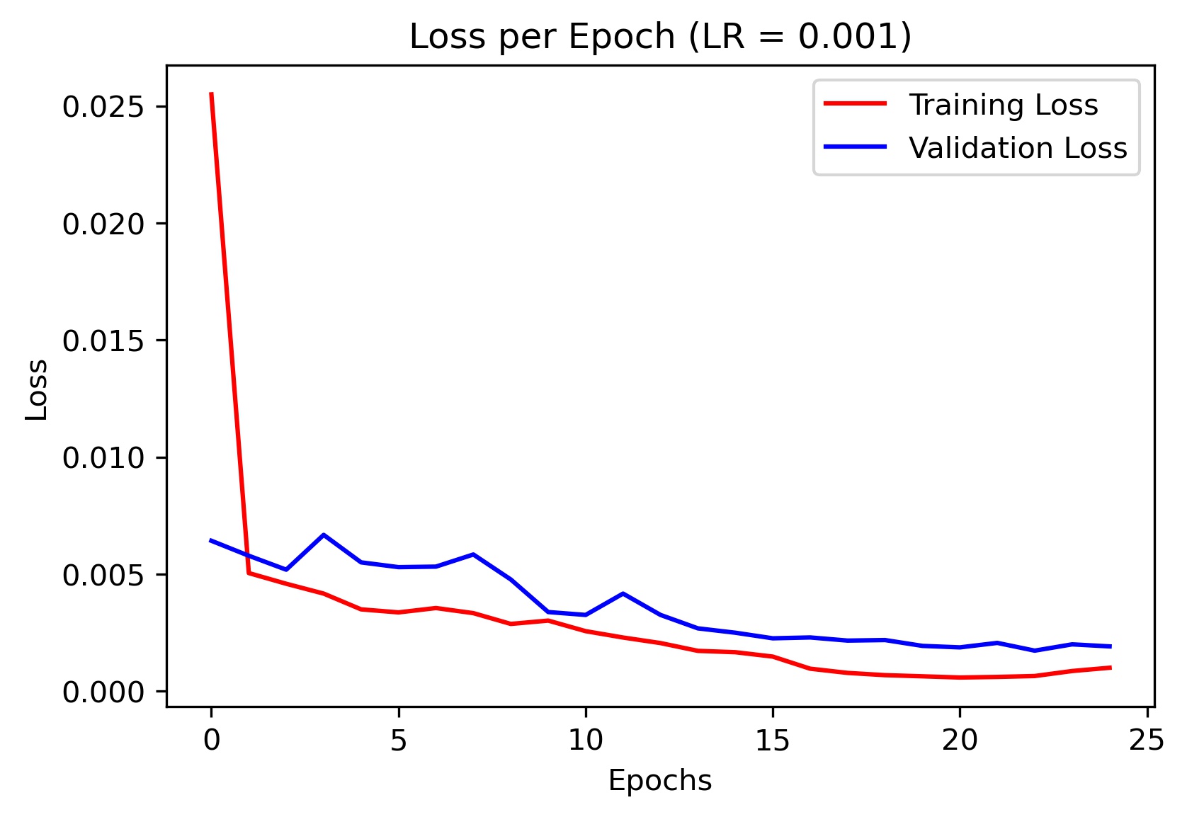
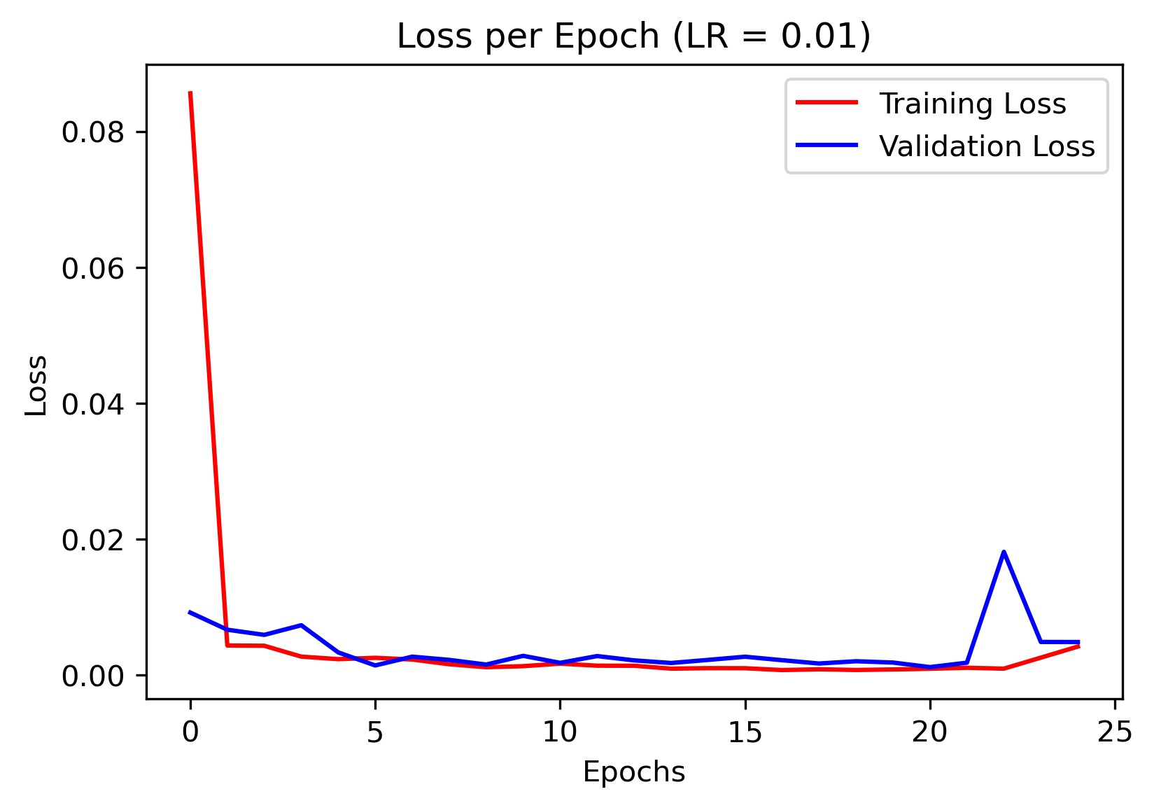
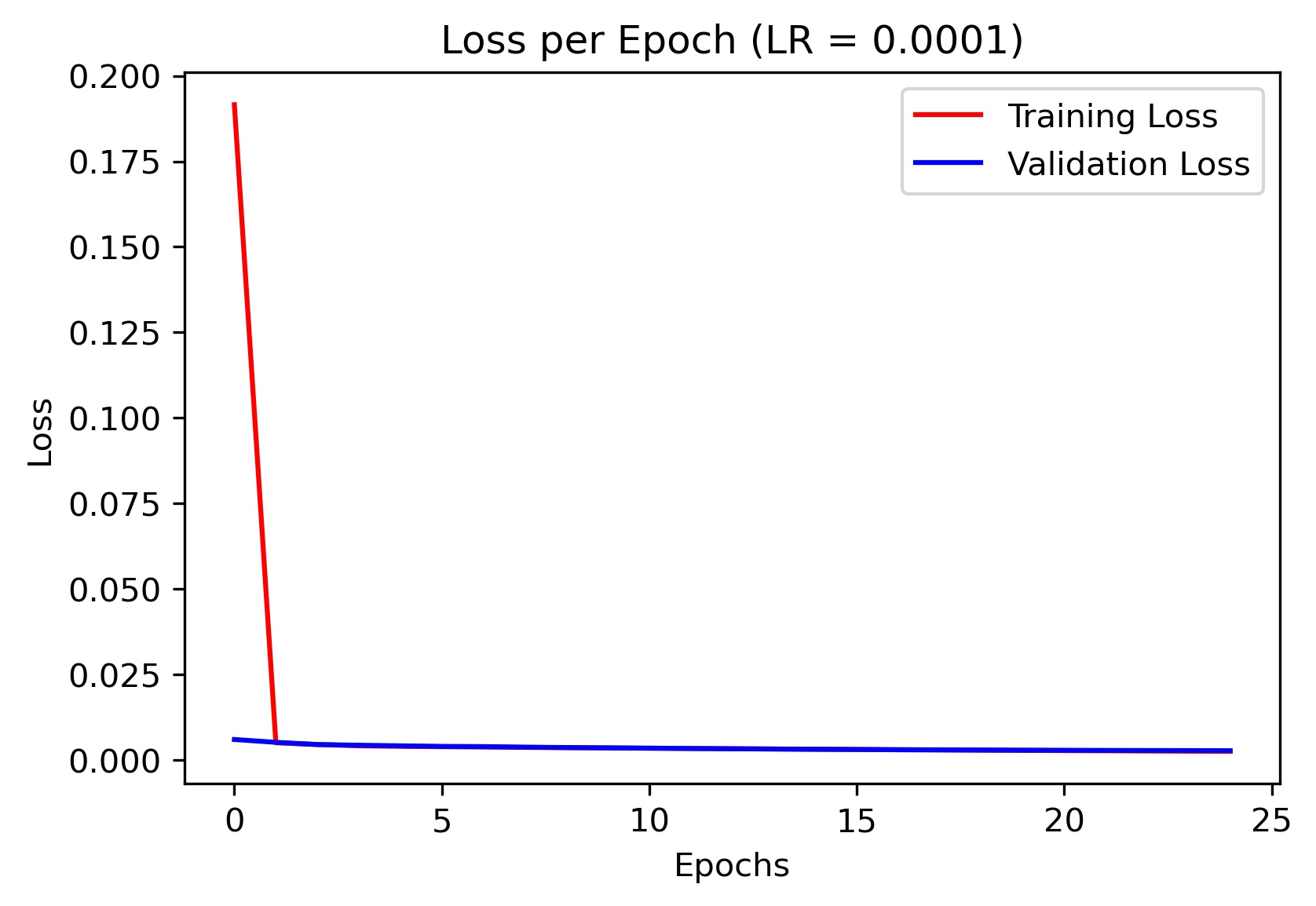
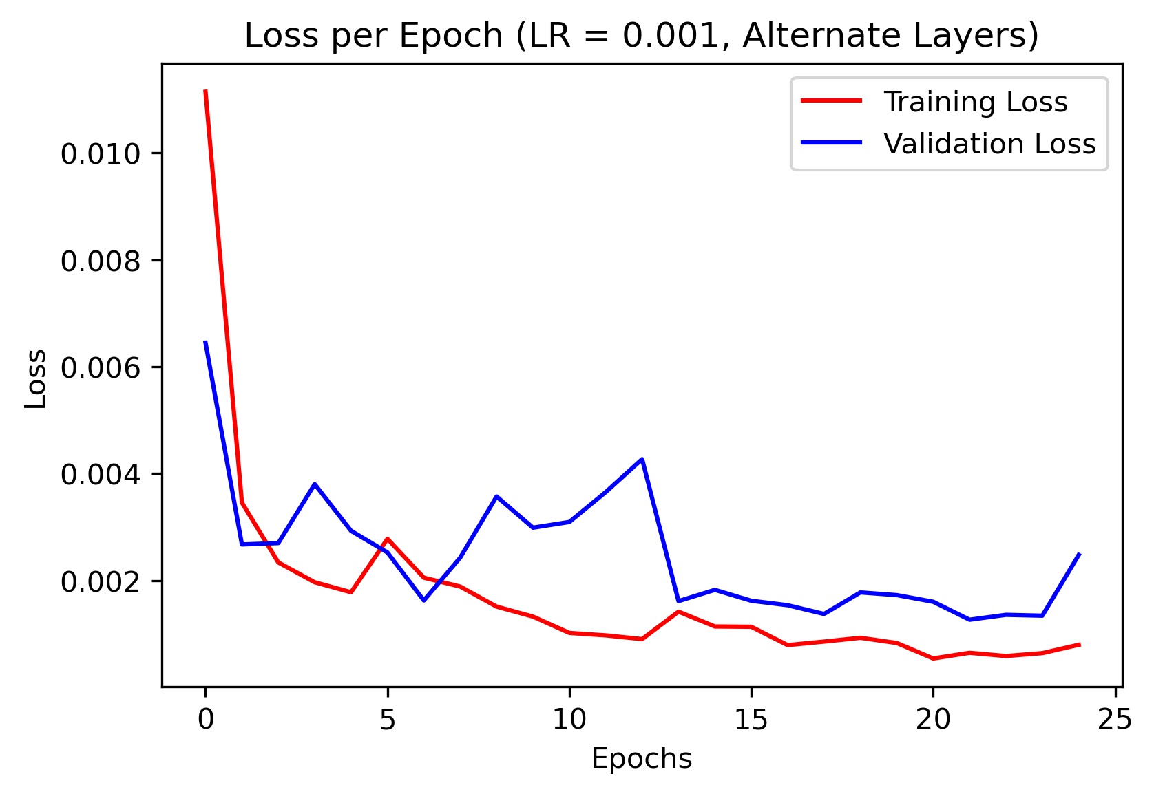
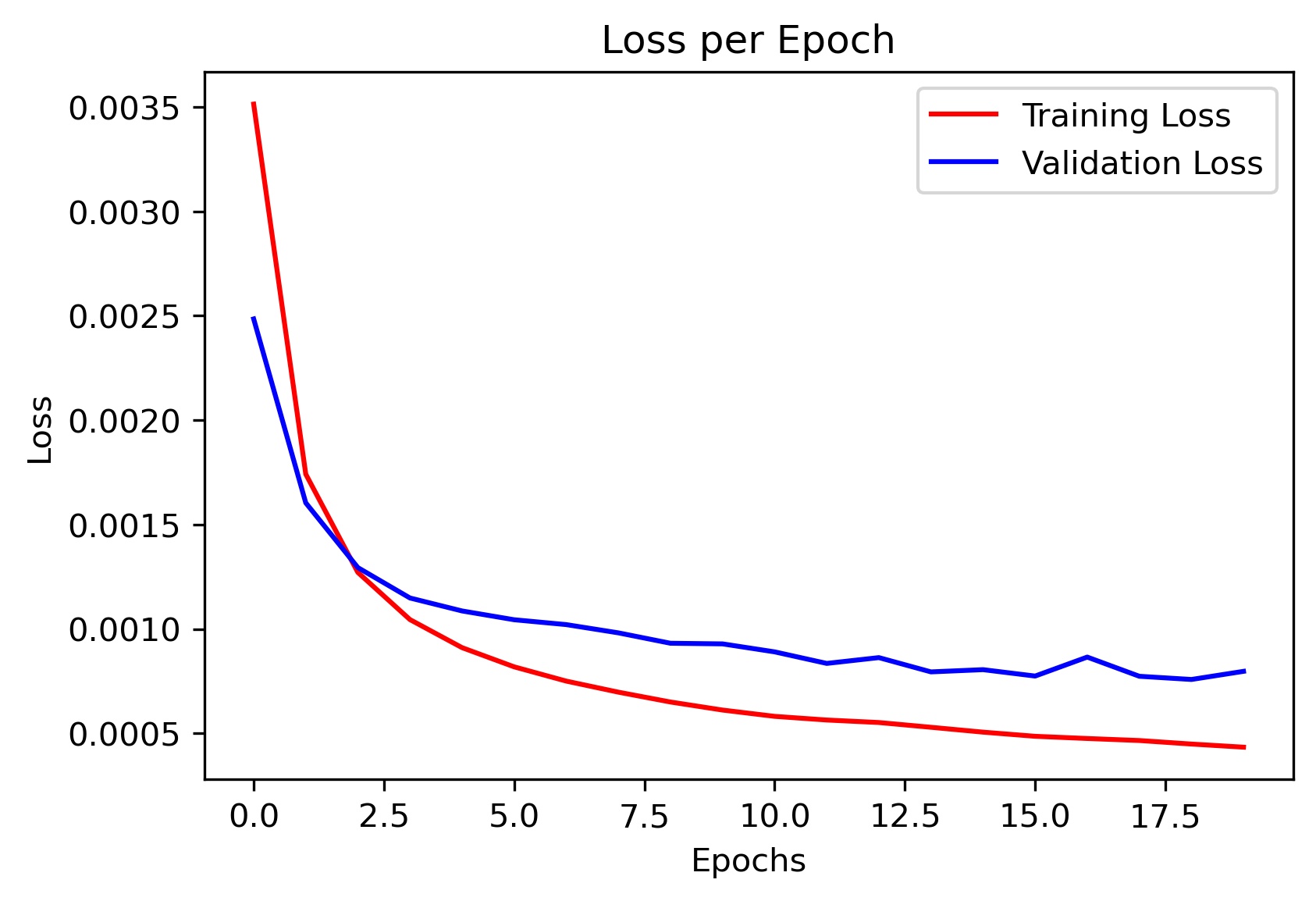
Here is the loss plot for different learning rates (I ended up using the model trained with learning rate of 0.001 for my final results):
|
|
|
I experimented with a few different choices of hyperparameters, such as changing kernel sizes in the convolutional layers, changing the number of max pools, and changing the learning rate. Here is an alternate model architecture I tried:
            SimpleCNN(
                (layer1): Sequential(
                (0): Conv2d(1, 16, kernel_size=(3, 3), stride=(1, 1))
                (1): ReLU()
                (2): MaxPool2d(kernel_size=2, stride=2, padding=0, dilation=1, ceil_mode=False)
                )
                (layer2): Sequential(
                (0): Conv2d(16, 32, kernel_size=(3, 3), stride=(1, 1))
                (1): ReLU()
                (2): MaxPool2d(kernel_size=2, stride=2, padding=0, dilation=1, ceil_mode=False)
                )
                (layer3): Sequential(
                (0): Conv2d(32, 16, kernel_size=(5, 5), stride=(1, 1))
                (1): ReLU()
                (2): MaxPool2d(kernel_size=2, stride=2, padding=0, dilation=1, ceil_mode=False)
                )
                (layer4): Sequential(
                (0): Conv2d(16, 12, kernel_size=(3, 3), stride=(1, 1))
                (1): ReLU()
                (2): MaxPool2d(kernel_size=2, stride=2, padding=0, dilation=1, ceil_mode=False)
                )
                (layer5): Sequential(
                (0): Flatten(start_dim=1, end_dim=-1)
                (1): Linear(in_features=2112, out_features=500, bias=True)
                (2): ReLU()
                )
                (layer6): Sequential(
                (0): Linear(in_features=500, out_features=2, bias=True)
                )
            )
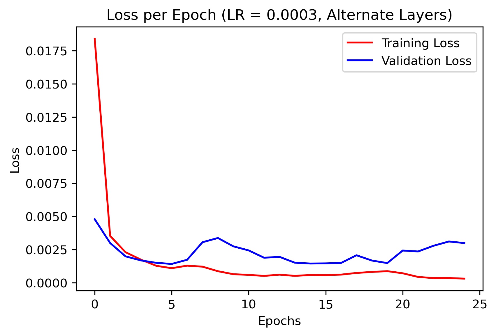
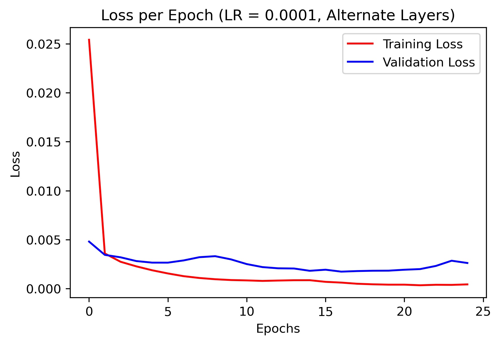
To test the efficacy of this alternate architecture, I plotted the training and validation loss for various learning rates. Here are the results:
|
|
|
As evidenced by the plots, the original architecture performed the best at generalizing.
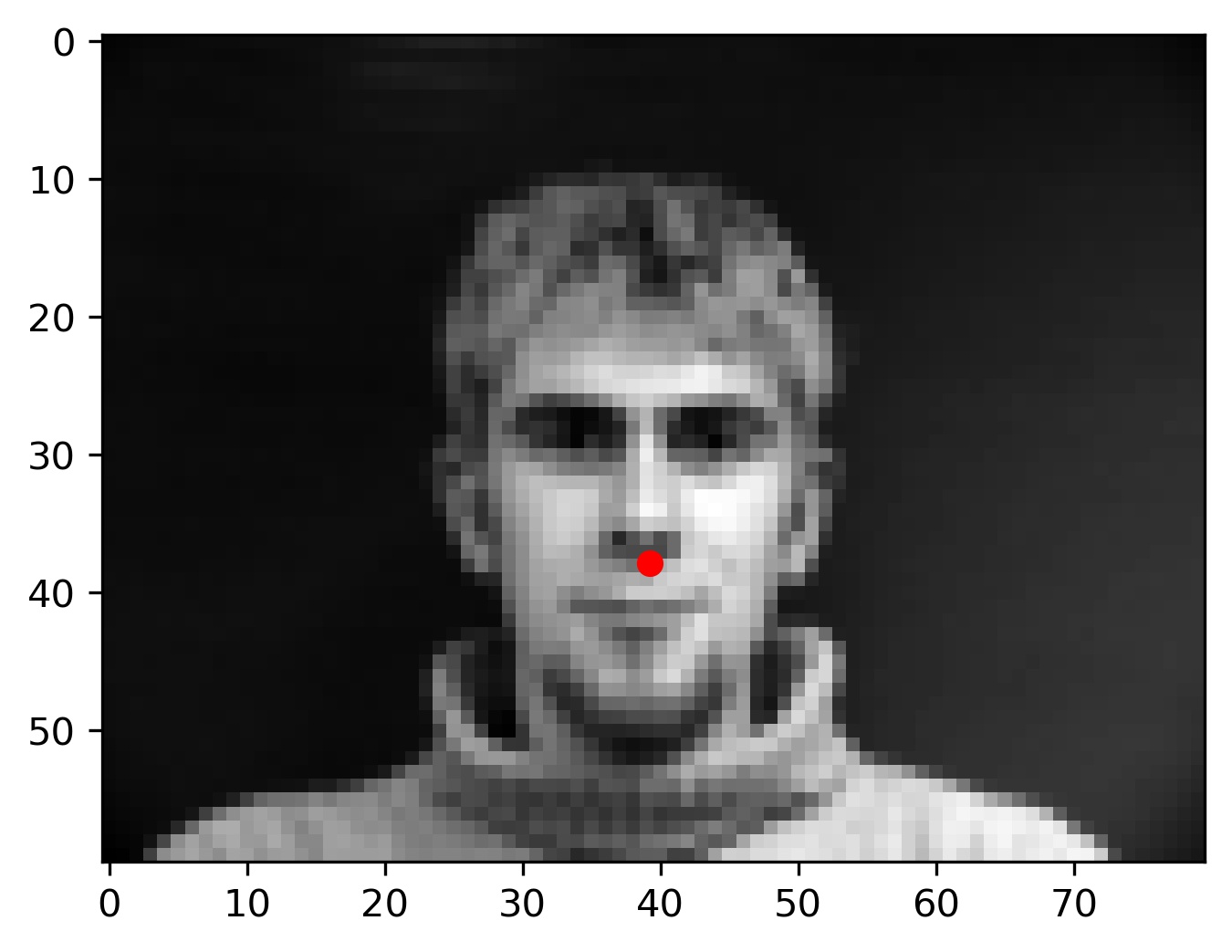
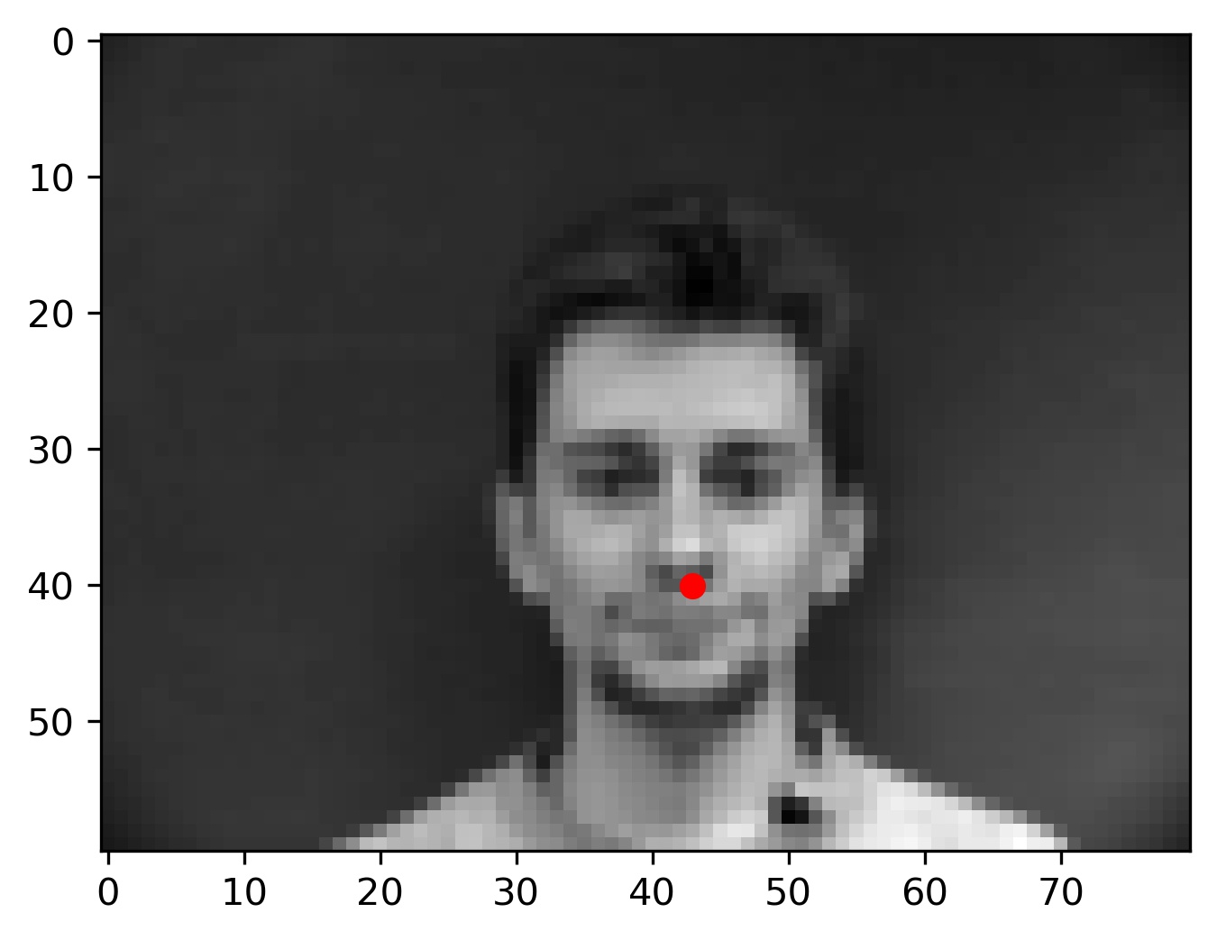
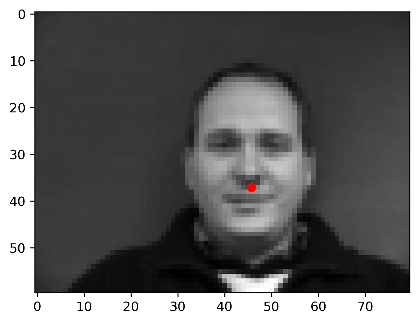
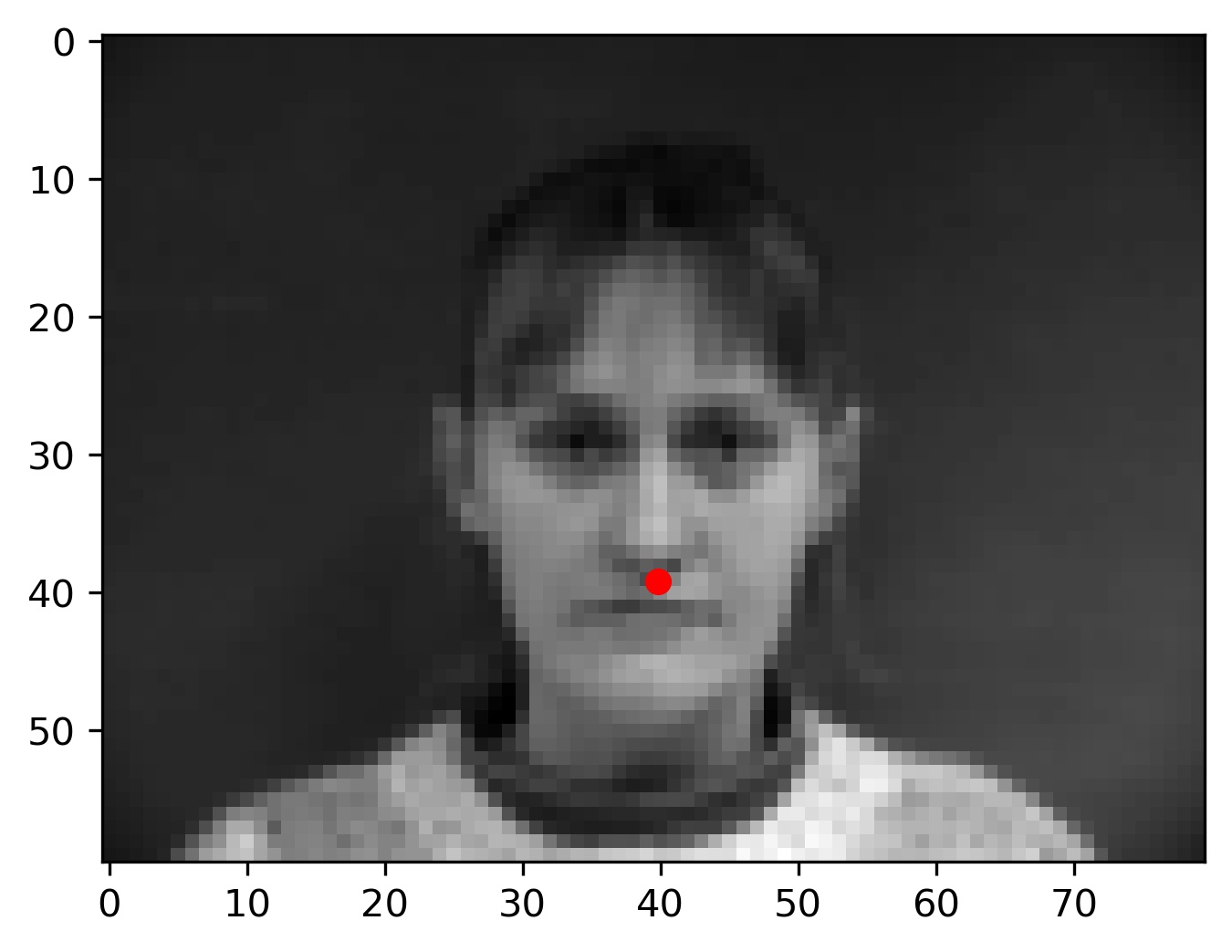
Here are some of the results from my model:
|
|
|
|
|
|
Notice that in failure cases 2 and 3, the faces are tilted to the side as opposed to facing the camera face on. The model's inability to classify these points correctly is likely attributed to a lack of training data with examples of this form. This can be combatted by getting more images, or by using data augmentation.
Part 2 - Simple Full Face Keypoint Classification
This part of the project is very similar to part 1, except we now seek classify 68 keypoints of a face instead of just the nose.
For the data loader, we now implement naive data augmentation. This augmentation includes random rotation, and random shifts. Here are some examples from the data loader:
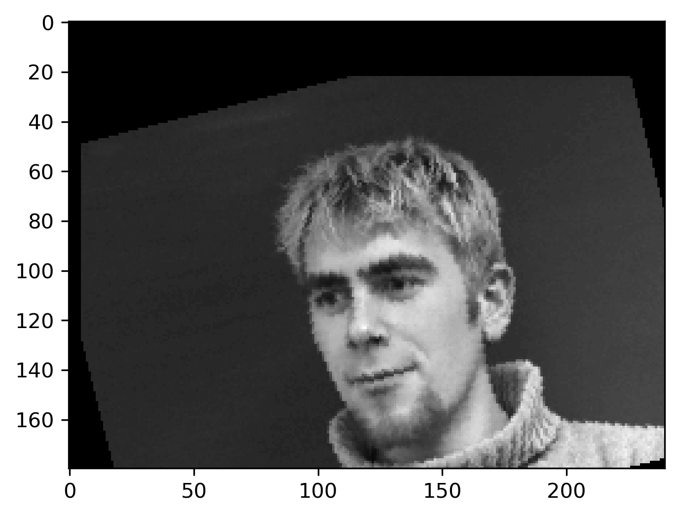
|
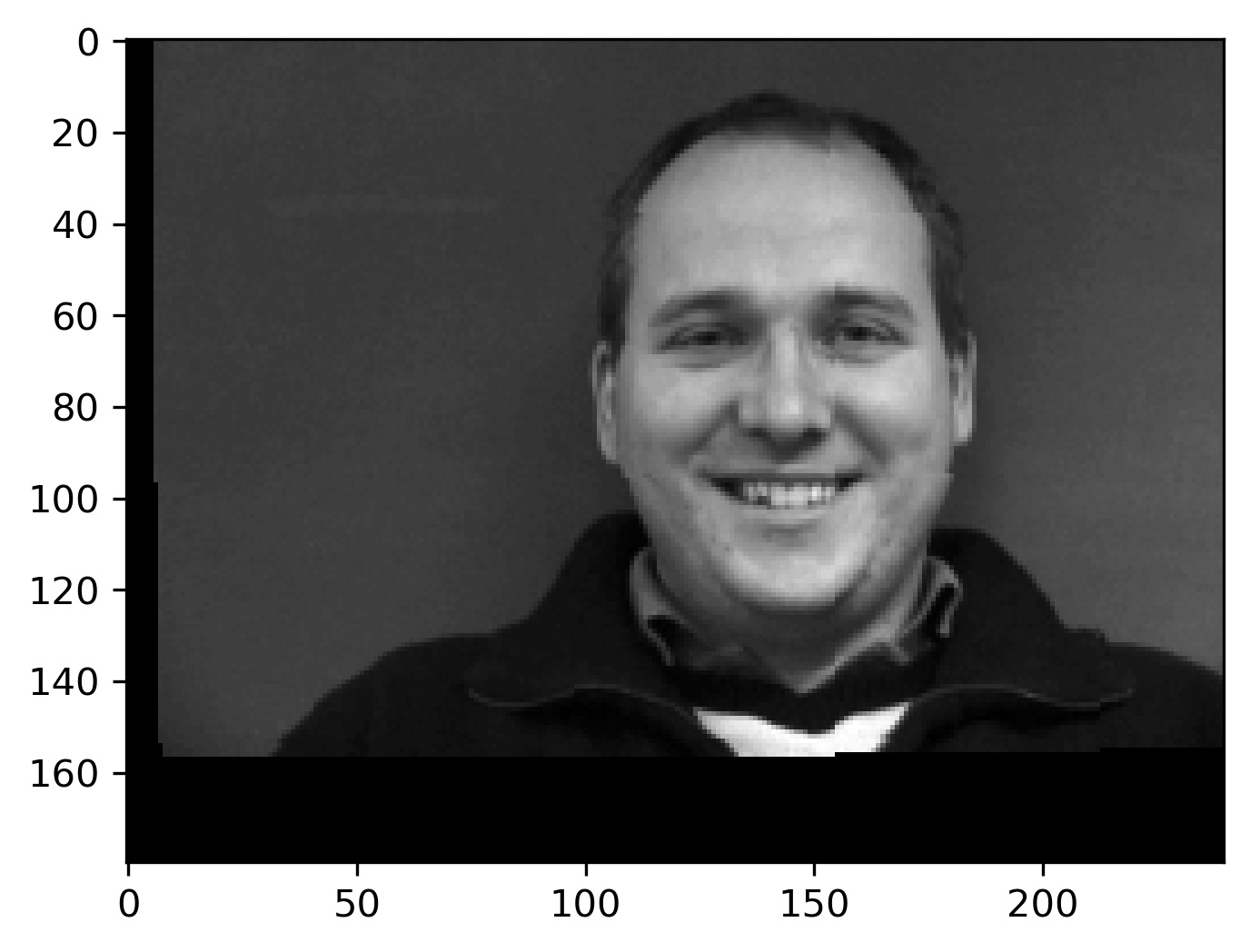
|
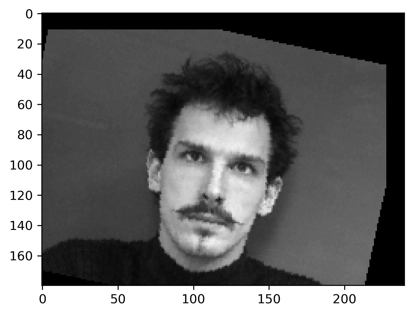
|
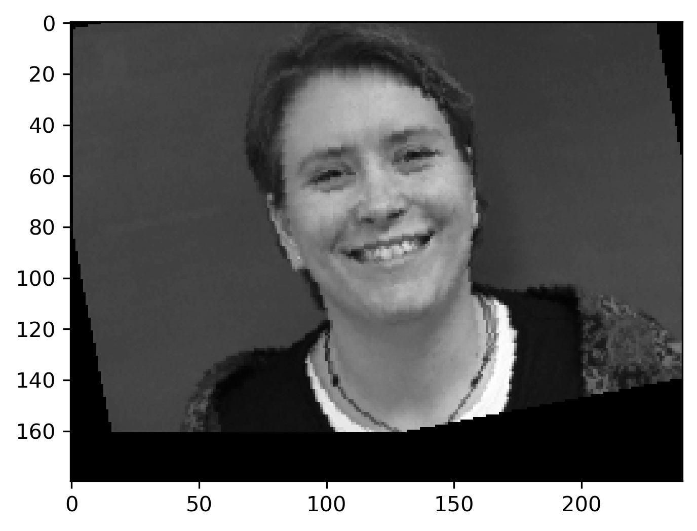
|
My final model architecture for part 2 is as follows:
            FullFaceCNN(
                (layer1): Sequential(
                    (0): Conv2d(1, 8, kernel_size=(3, 3), stride=(1, 1))
                    (1): ReLU()
                )
                (layer2): Sequential(
                    (0): Conv2d(8, 8, kernel_size=(3, 3), stride=(1, 1))
                    (1): ReLU()
                )
                (layer3): Sequential(
                    (0): Conv2d(8, 8, kernel_size=(3, 3), stride=(2, 2))
                    (1): ReLU()
                )
                (layer4): Sequential(
                    (0): Conv2d(8, 8, kernel_size=(3, 3), stride=(2, 2))
                    (1): ReLU()
                )
                (layer5): Sequential(
                    (0): Conv2d(32, 16, kernel_size=(5, 5), stride=(1, 1))
                    (1): ReLU()
                    (2): MaxPool2d(kernel_size=2, stride=2, padding=0, dilation=1, ceil_mode=False)
                )
                (layer6): Sequential(
                    (0): Conv2d(16, 12, kernel_size=(3, 3), stride=(1, 1))
                    (1): ReLU()
                    (2): MaxPool2d(kernel_size=2, stride=2, padding=0, dilation=1, ceil_mode=False)
                )
                (layer7): Sequential(
                    (0): Flatten(start_dim=1, end_dim=-1)
                    (1): Linear(in_features=19952, out_features=500, bias=True)
                    (2): ReLU()
                )
                (layer8): Sequential(
                    (0): Linear(in_features=500, out_features=116, bias=True)
                )
            )
Here is the loss plot:
Here are some of the results from my model (notice that the model fails in similar situations as the model from part 1):
|
|
|
|
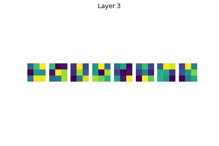
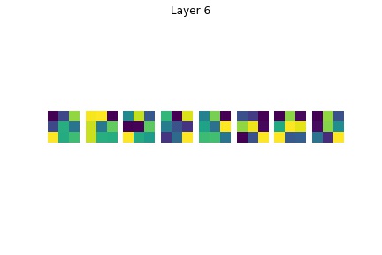
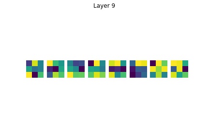
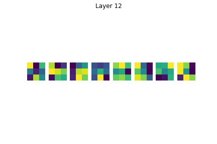
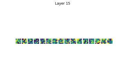
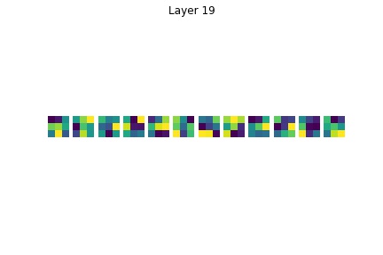
We can also try to visualize the features. Unfortunately, the meaning behind these is not super clear, but here they are anyways:
Part 3 - Train With More Data
In this part of the project, we have the same objective as in part 2 except that we have more data available to us. We also had to submit a set of predictions for a kaggle competition. I started with a naive architecture which is what I discuss in this section, however the final architecture that I used for my submission is covered in the bells and whistles section.
I used a modified Resnet-18 architecture as follows:
            ResNet(
                (conv1): Conv2d(1, 64, kernel_size=(7, 7), stride=(2, 2), padding=(3, 3), bias=False)
                (bn1): BatchNorm2d(64, eps=1e-05, momentum=0.1, affine=True, track_running_stats=True)
                (relu): ReLU(inplace=True)
                (maxpool): MaxPool2d(kernel_size=3, stride=2, padding=1, dilation=1, ceil_mode=False)
                (layer1): Sequential(
                    (0): BasicBlock(
                    (conv1): Conv2d(64, 64, kernel_size=(3, 3), stride=(1, 1), padding=(1, 1), bias=False)
                    (bn1): BatchNorm2d(64, eps=1e-05, momentum=0.1, affine=True, track_running_stats=True)
                    (relu): ReLU(inplace=True)
                    (conv2): Conv2d(64, 64, kernel_size=(3, 3), stride=(1, 1), padding=(1, 1), bias=False)
                    (bn2): BatchNorm2d(64, eps=1e-05, momentum=0.1, affine=True, track_running_stats=True)
                    )
                    (1): BasicBlock(
                    (conv1): Conv2d(64, 64, kernel_size=(3, 3), stride=(1, 1), padding=(1, 1), bias=False)
                    (bn1): BatchNorm2d(64, eps=1e-05, momentum=0.1, affine=True, track_running_stats=True)
                    (relu): ReLU(inplace=True)
                    (conv2): Conv2d(64, 64, kernel_size=(3, 3), stride=(1, 1), padding=(1, 1), bias=False)
                    (bn2): BatchNorm2d(64, eps=1e-05, momentum=0.1, affine=True, track_running_stats=True)
                    )
                )
                (layer2): Sequential(
                    (0): BasicBlock(
                    (conv1): Conv2d(64, 128, kernel_size=(3, 3), stride=(2, 2), padding=(1, 1), bias=False)
                    (bn1): BatchNorm2d(128, eps=1e-05, momentum=0.1, affine=True, track_running_stats=True)
                    (relu): ReLU(inplace=True)
                    (conv2): Conv2d(128, 128, kernel_size=(3, 3), stride=(1, 1), padding=(1, 1), bias=False)
                    (bn2): BatchNorm2d(128, eps=1e-05, momentum=0.1, affine=True, track_running_stats=True)
                    (downsample): Sequential(
                        (0): Conv2d(64, 128, kernel_size=(1, 1), stride=(2, 2), bias=False)
                        (1): BatchNorm2d(128, eps=1e-05, momentum=0.1, affine=True, track_running_stats=True)
                    )
                    )
                    (1): BasicBlock(
                    (conv1): Conv2d(128, 128, kernel_size=(3, 3), stride=(1, 1), padding=(1, 1), bias=False)
                    (bn1): BatchNorm2d(128, eps=1e-05, momentum=0.1, affine=True, track_running_stats=True)
                    (relu): ReLU(inplace=True)
                    (conv2): Conv2d(128, 128, kernel_size=(3, 3), stride=(1, 1), padding=(1, 1), bias=False)
                    (bn2): BatchNorm2d(128, eps=1e-05, momentum=0.1, affine=True, track_running_stats=True)
                    )
                )
                (layer3): Sequential(
                    (0): BasicBlock(
                    (conv1): Conv2d(128, 256, kernel_size=(3, 3), stride=(2, 2), padding=(1, 1), bias=False)
                    (bn1): BatchNorm2d(256, eps=1e-05, momentum=0.1, affine=True, track_running_stats=True)
                    (relu): ReLU(inplace=True)
                    (conv2): Conv2d(256, 256, kernel_size=(3, 3), stride=(1, 1), padding=(1, 1), bias=False)
                    (bn2): BatchNorm2d(256, eps=1e-05, momentum=0.1, affine=True, track_running_stats=True)
                    (downsample): Sequential(
                        (0): Conv2d(128, 256, kernel_size=(1, 1), stride=(2, 2), bias=False)
                        (1): BatchNorm2d(256, eps=1e-05, momentum=0.1, affine=True, track_running_stats=True)
                    )
                    )
                    (1): BasicBlock(
                    (conv1): Conv2d(256, 256, kernel_size=(3, 3), stride=(1, 1), padding=(1, 1), bias=False)
                    (bn1): BatchNorm2d(256, eps=1e-05, momentum=0.1, affine=True, track_running_stats=True)
                    (relu): ReLU(inplace=True)
                    (conv2): Conv2d(256, 256, kernel_size=(3, 3), stride=(1, 1), padding=(1, 1), bias=False)
                    (bn2): BatchNorm2d(256, eps=1e-05, momentum=0.1, affine=True, track_running_stats=True)
                    )
                )
                (layer4): Sequential(
                    (0): BasicBlock(
                    (conv1): Conv2d(256, 512, kernel_size=(3, 3), stride=(2, 2), padding=(1, 1), bias=False)
                    (bn1): BatchNorm2d(512, eps=1e-05, momentum=0.1, affine=True, track_running_stats=True)
                    (relu): ReLU(inplace=True)
                    (conv2): Conv2d(512, 512, kernel_size=(3, 3), stride=(1, 1), padding=(1, 1), bias=False)
                    (bn2): BatchNorm2d(512, eps=1e-05, momentum=0.1, affine=True, track_running_stats=True)
                    (downsample): Sequential(
                        (0): Conv2d(256, 512, kernel_size=(1, 1), stride=(2, 2), bias=False)
                        (1): BatchNorm2d(512, eps=1e-05, momentum=0.1, affine=True, track_running_stats=True)
                    )
                    )
                    (1): BasicBlock(
                    (conv1): Conv2d(512, 512, kernel_size=(3, 3), stride=(1, 1), padding=(1, 1), bias=False)
                    (bn1): BatchNorm2d(512, eps=1e-05, momentum=0.1, affine=True, track_running_stats=True)
                    (relu): ReLU(inplace=True)
                    (conv2): Conv2d(512, 512, kernel_size=(3, 3), stride=(1, 1), padding=(1, 1), bias=False)
                    (bn2): BatchNorm2d(512, eps=1e-05, momentum=0.1, affine=True, track_running_stats=True)
                    )
                )
                (avgpool): AdaptiveAvgPool2d(output_size=(1, 1))
                (fc): Linear(in_features=512, out_features=136, bias=True)
            )
Since I was not planning on using this model for my final submission, I did not train for that many epochs. The loss curve is given below:
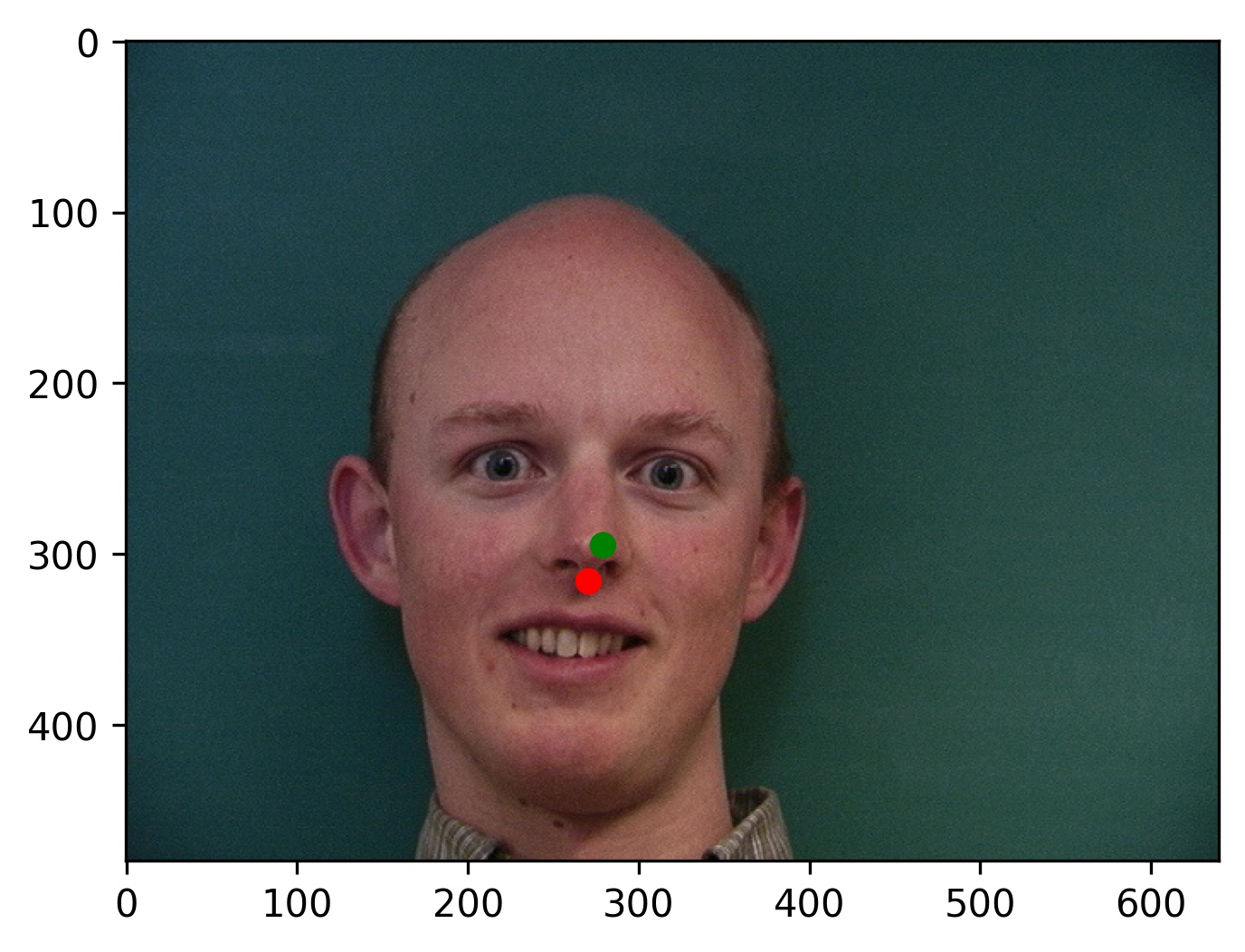
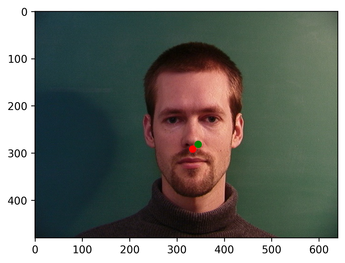
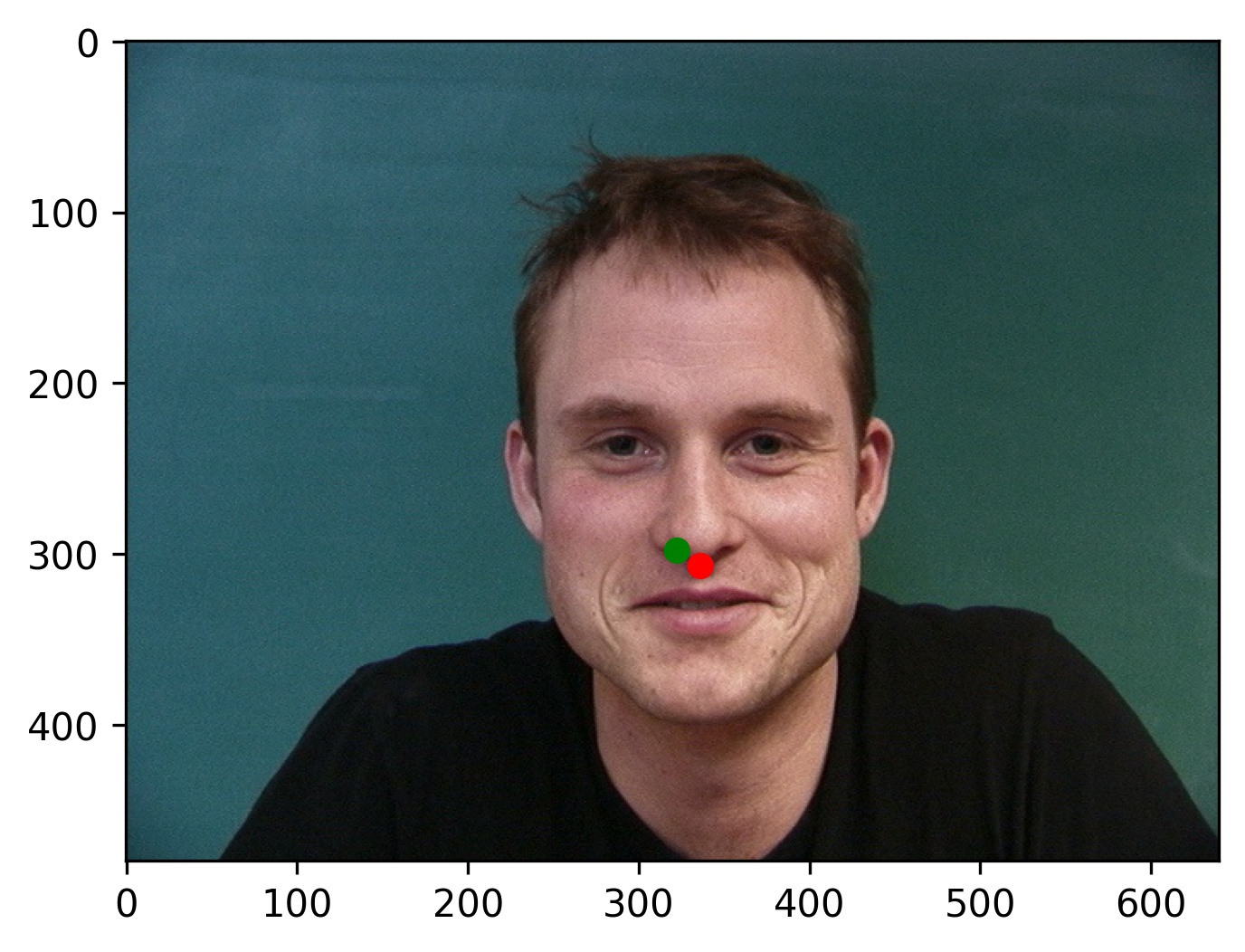
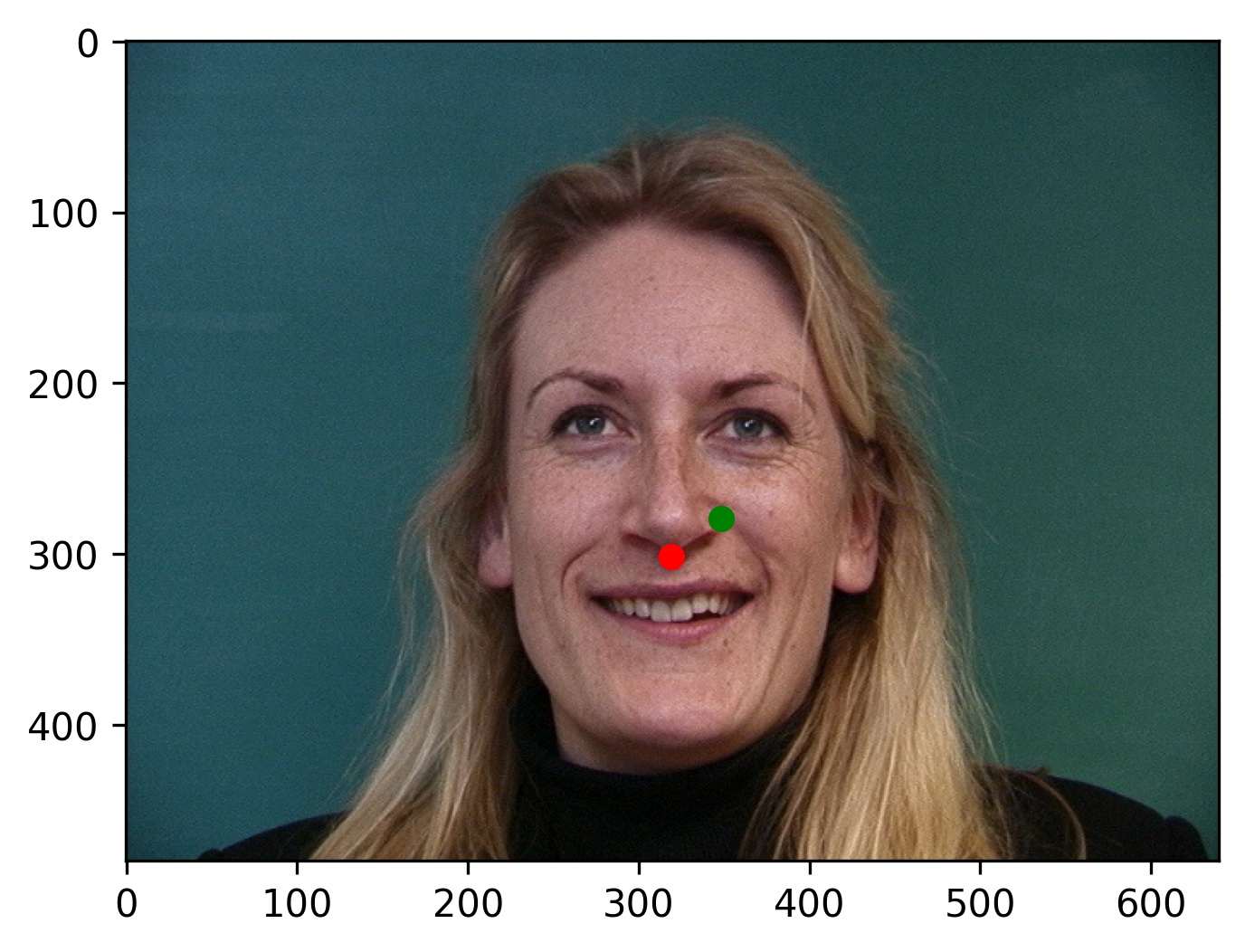
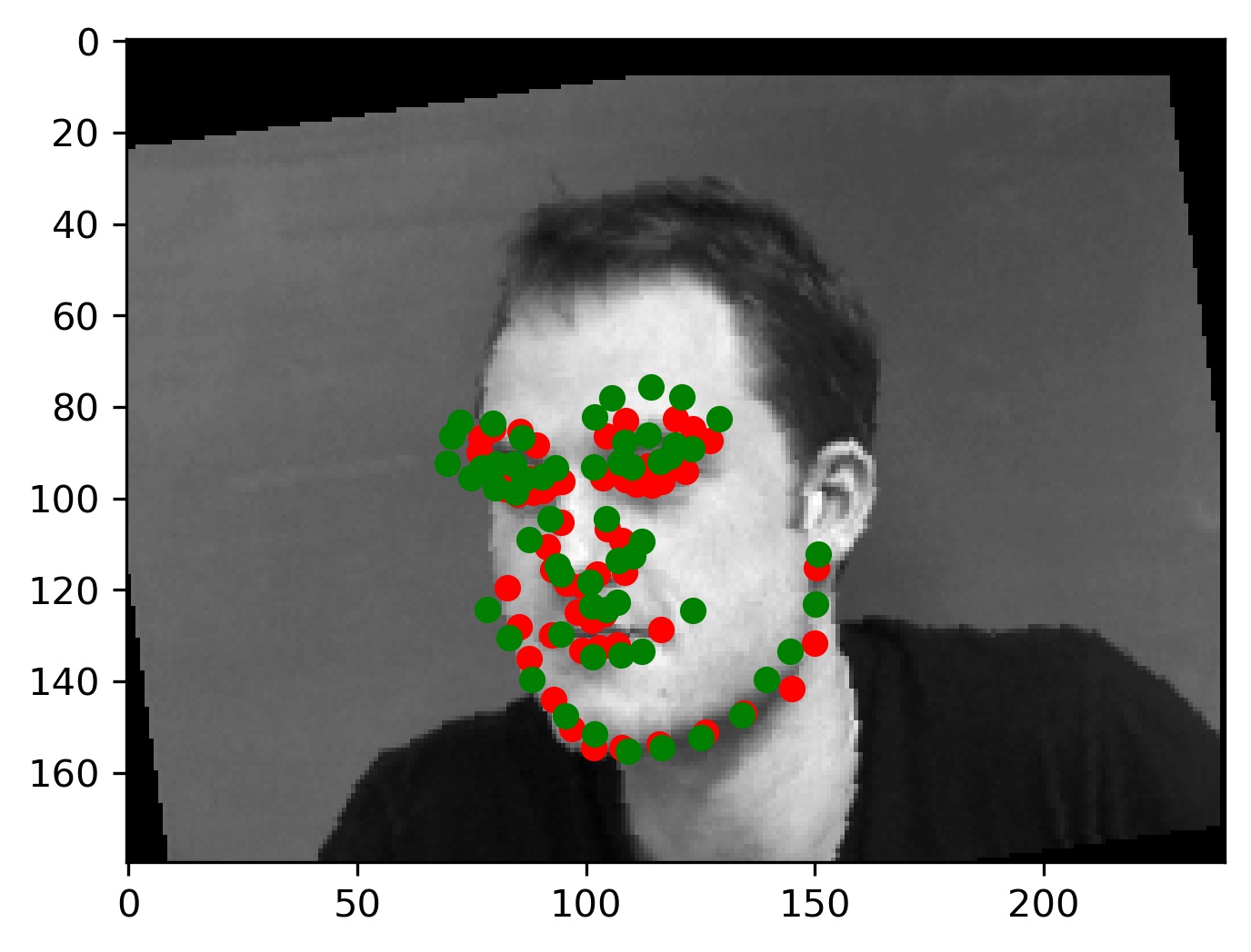
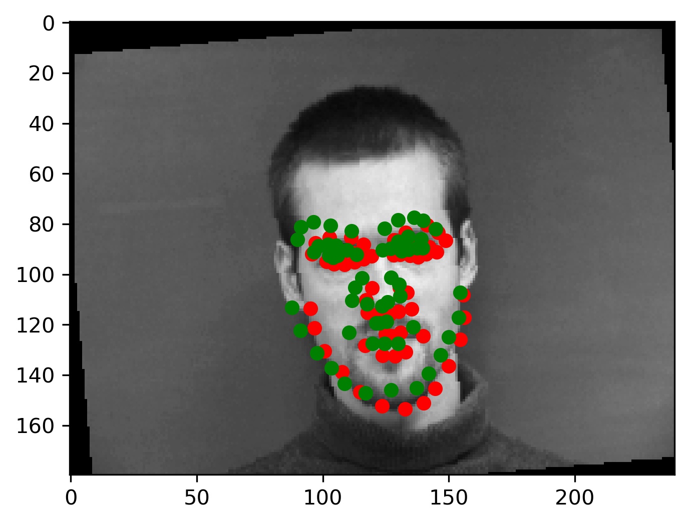
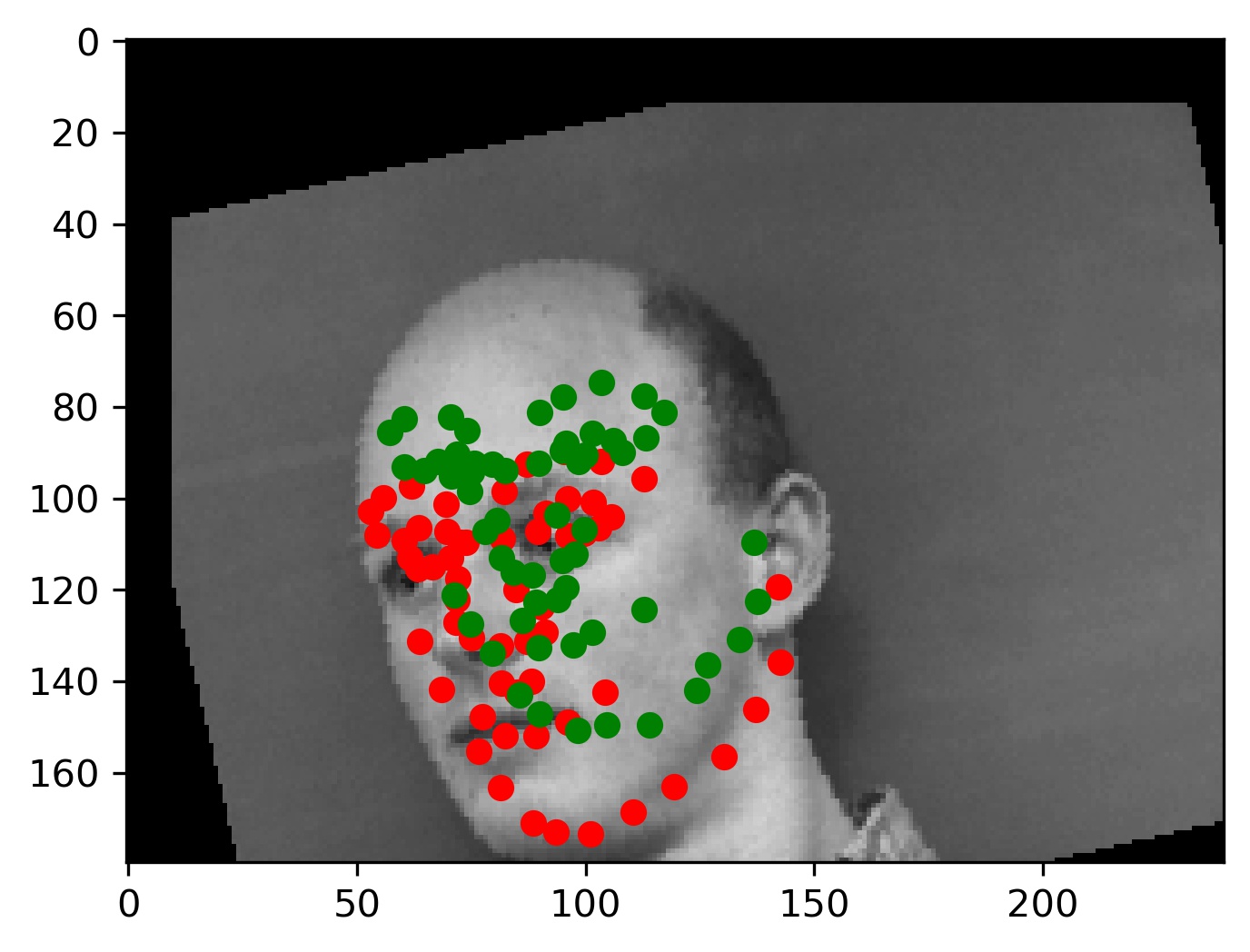
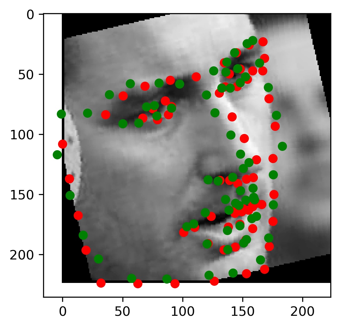
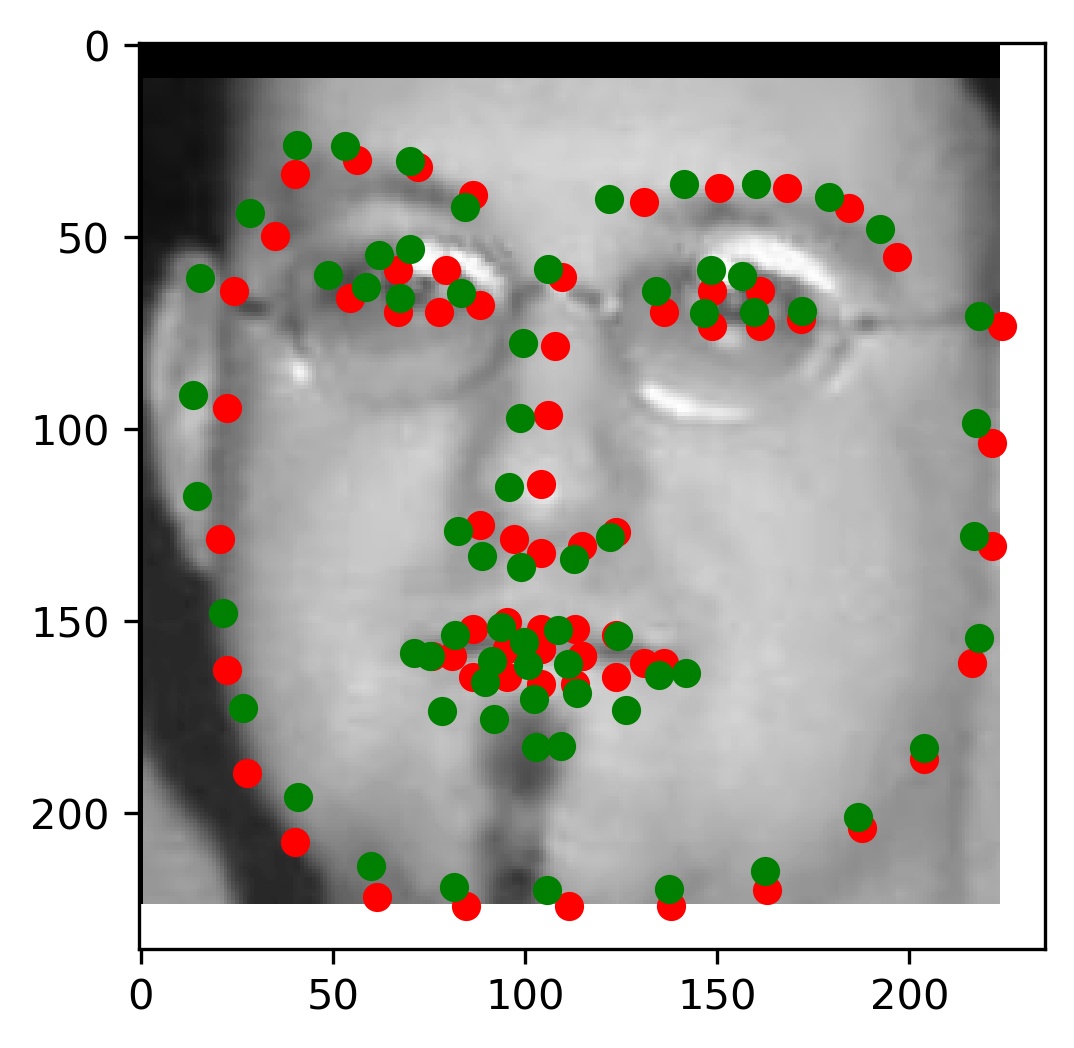
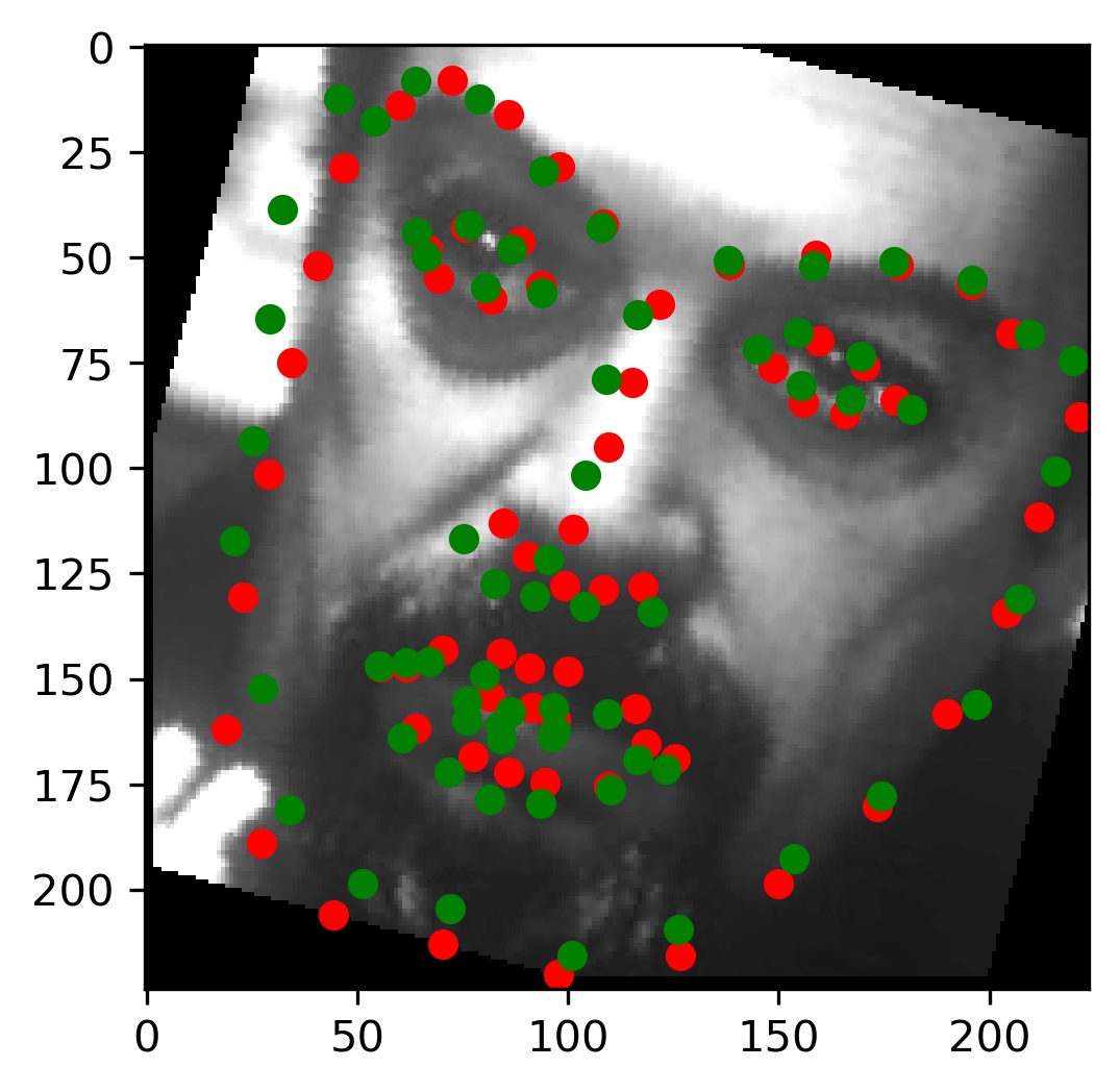
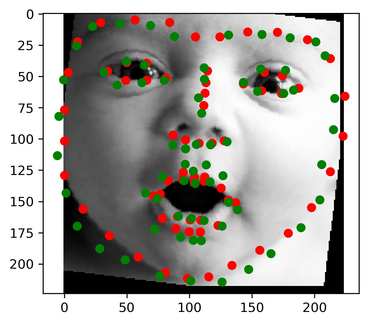
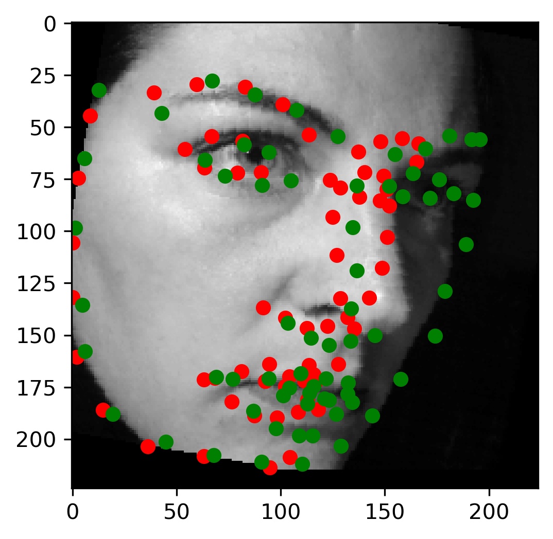
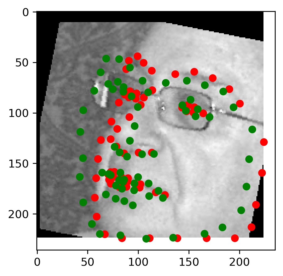
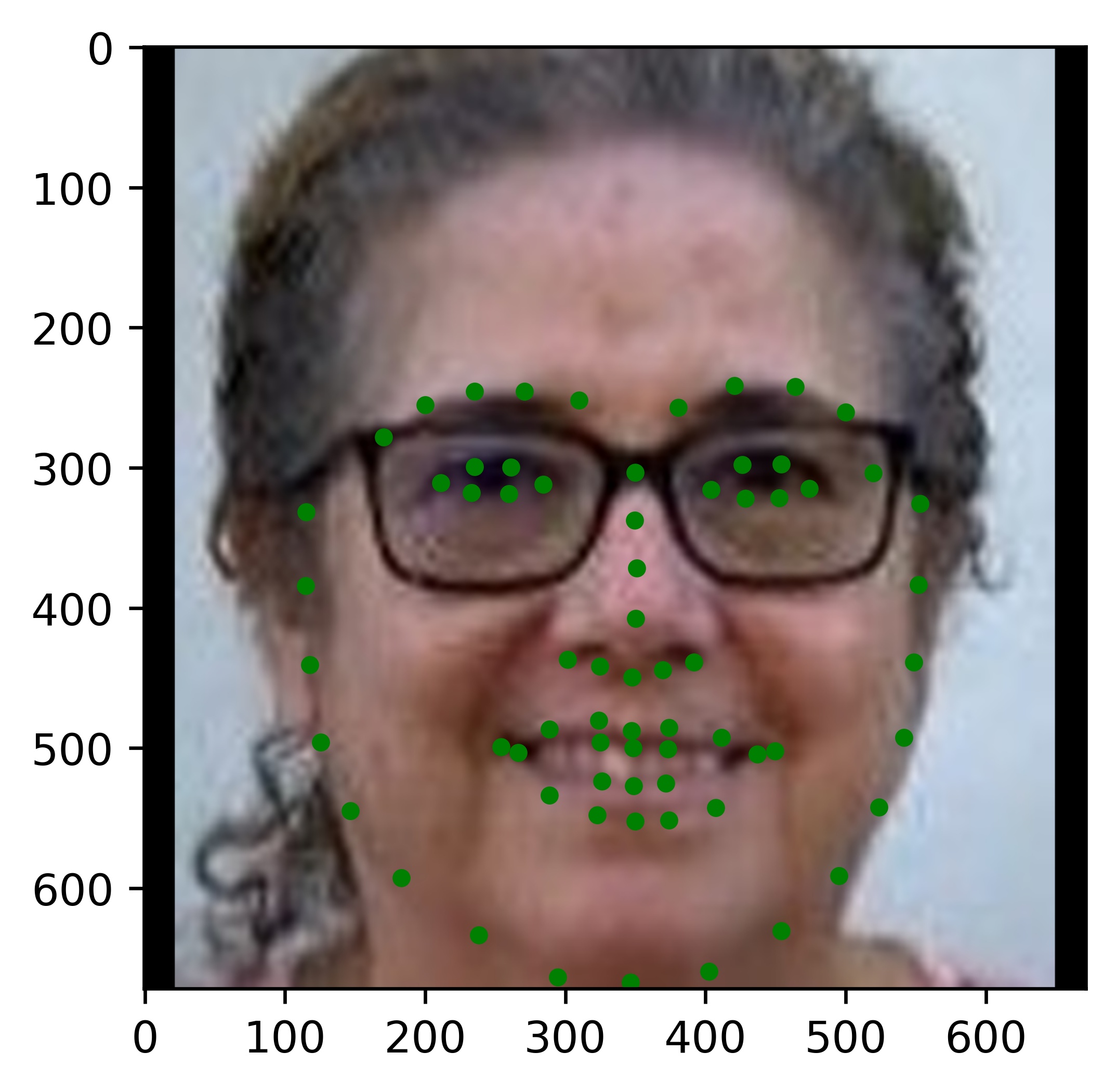
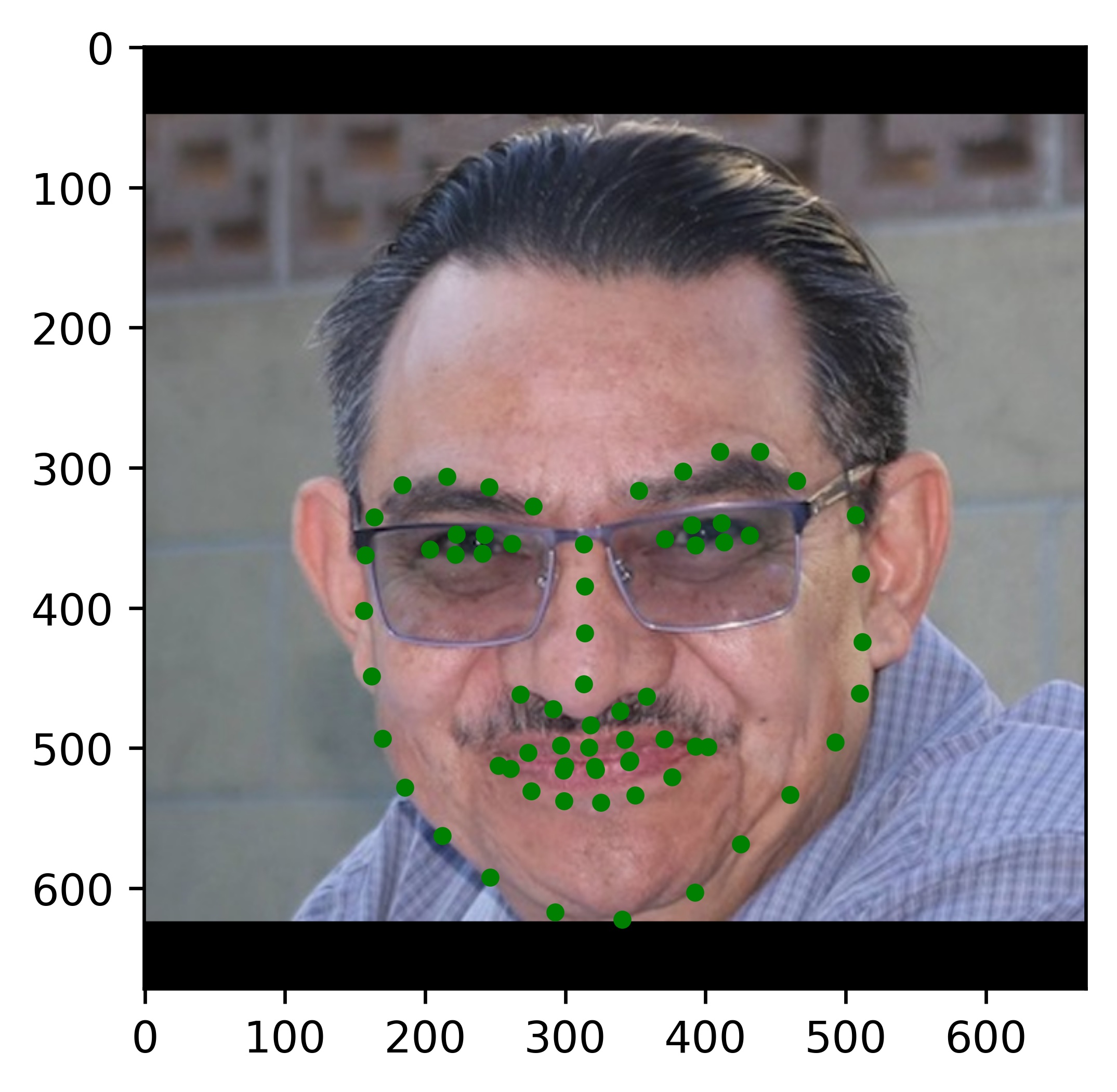
This model performed decent, and certainly could have done better with more training. Here are some results of the model on the validation set (note that red is the ground truth, and green is the prediction):
|
|
|
|
|
|
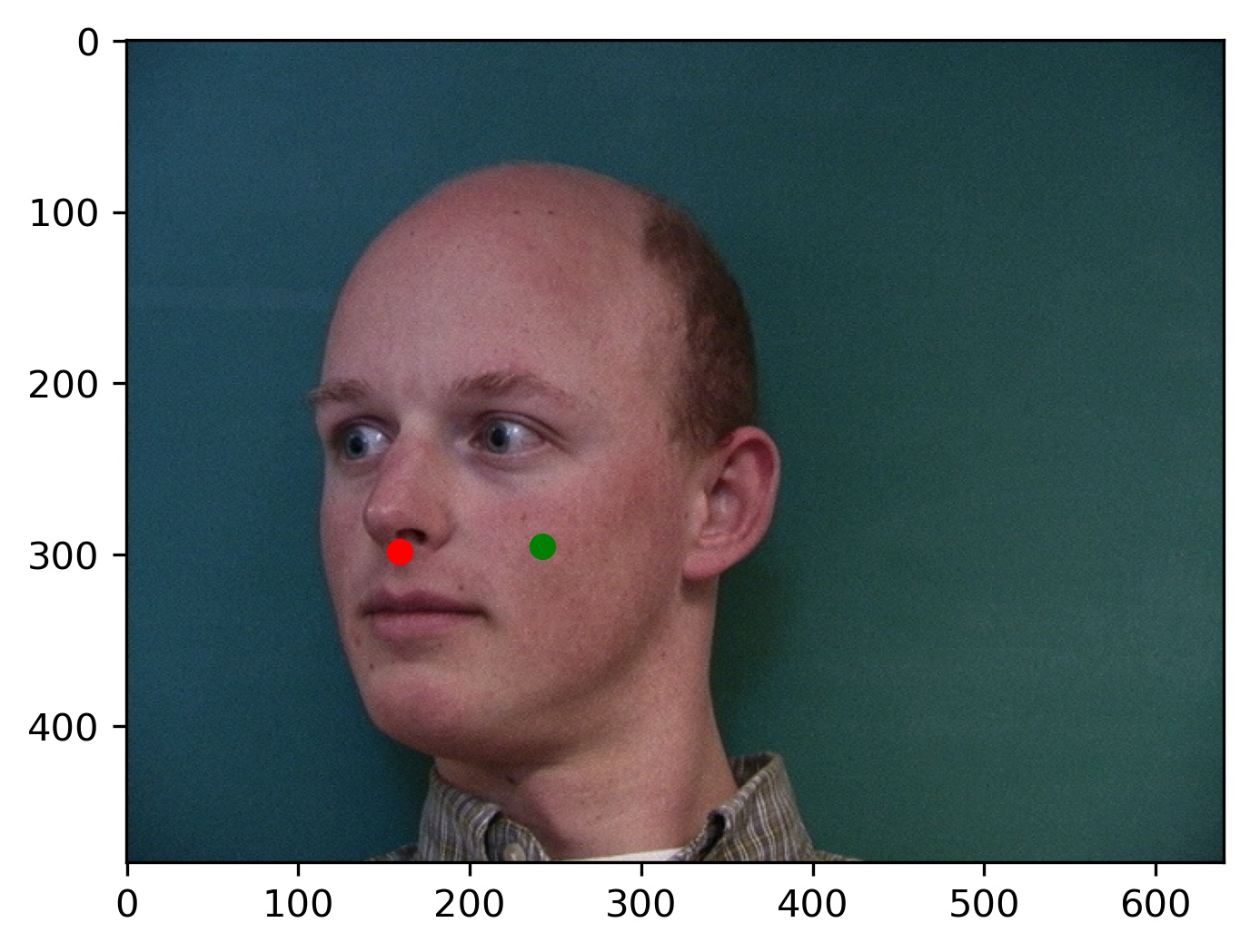
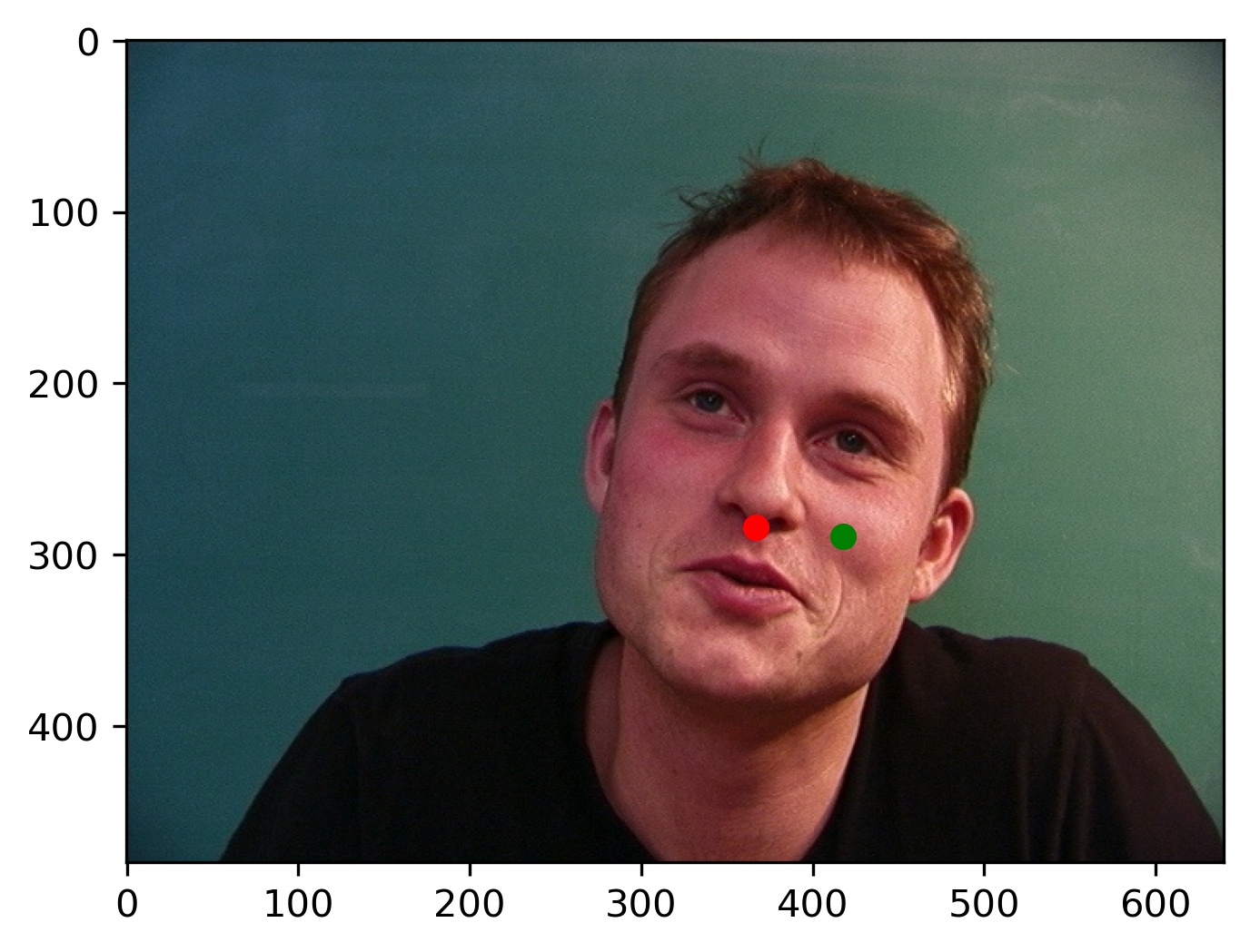
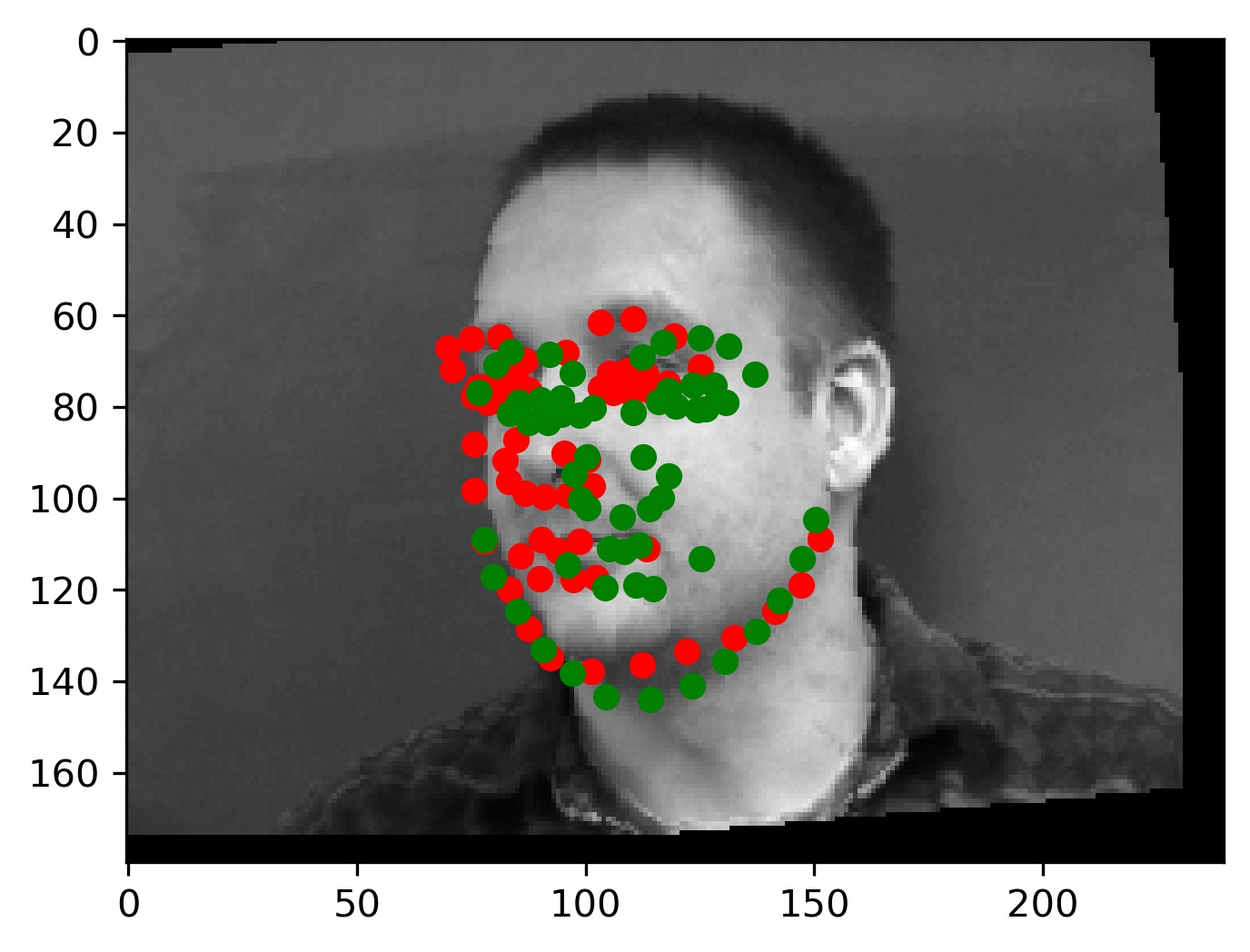
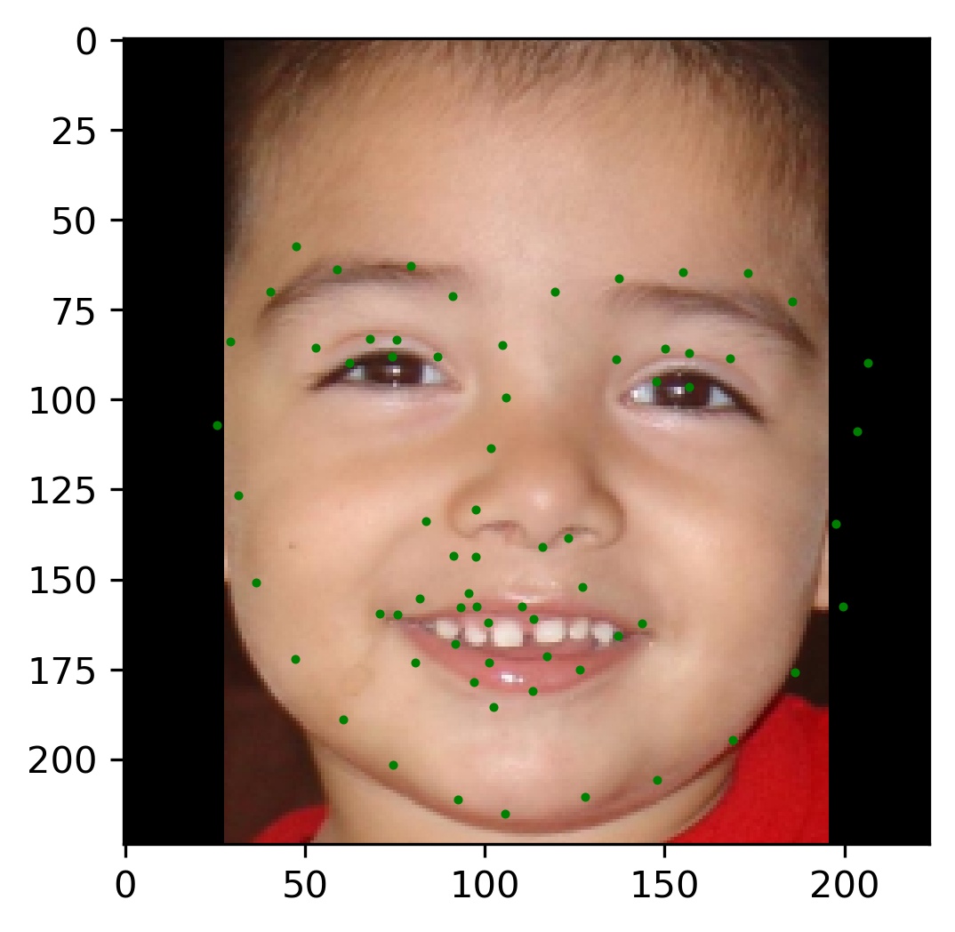
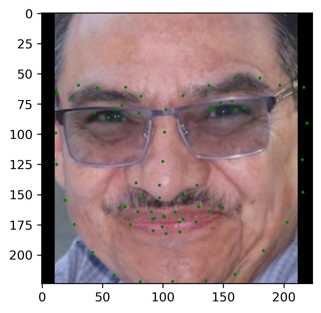
Finally, I ran the model on some of my own images. Here are those results:
|
|
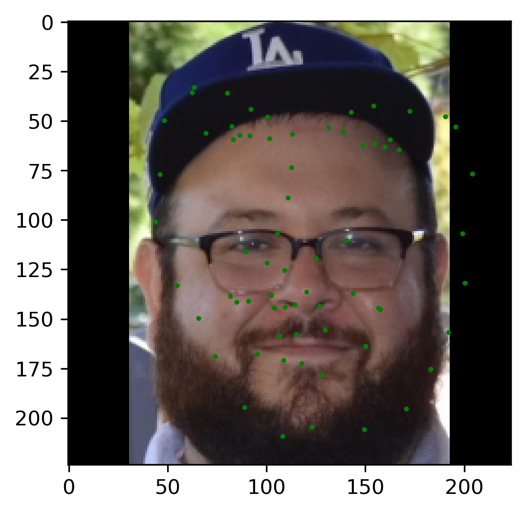
|
As you can see, the results are pretty good for images that are cropped to just the face. However, since I did not crop the picture for my brother, the results are not as good. This shows a failure of the model to generalize to poor bounding boxes. However, this is by design because every training image was perfectly cropped to the labeled bounding box. This is something I sought to address in the bells and whistles.
Bells and Whistles (The Fun Stuff)
Implementing UNET
One of the issues with using resnet 18 is that it was built primarily for classification. With this in mind, the architecture uses various pooling operations that takes away precious spacial precision from our model. Since spacial precision is everything for us, it is better to try an architecture that does not lose this information. We could consider simply removing some of the pooling layers, however this would come at the cost of making the model take much longer to train. The reason why is that pooling layers allow us to efficiently reduce the size of tensors throughout the network, and so removing them would greatly increase the number of learnable parameters.
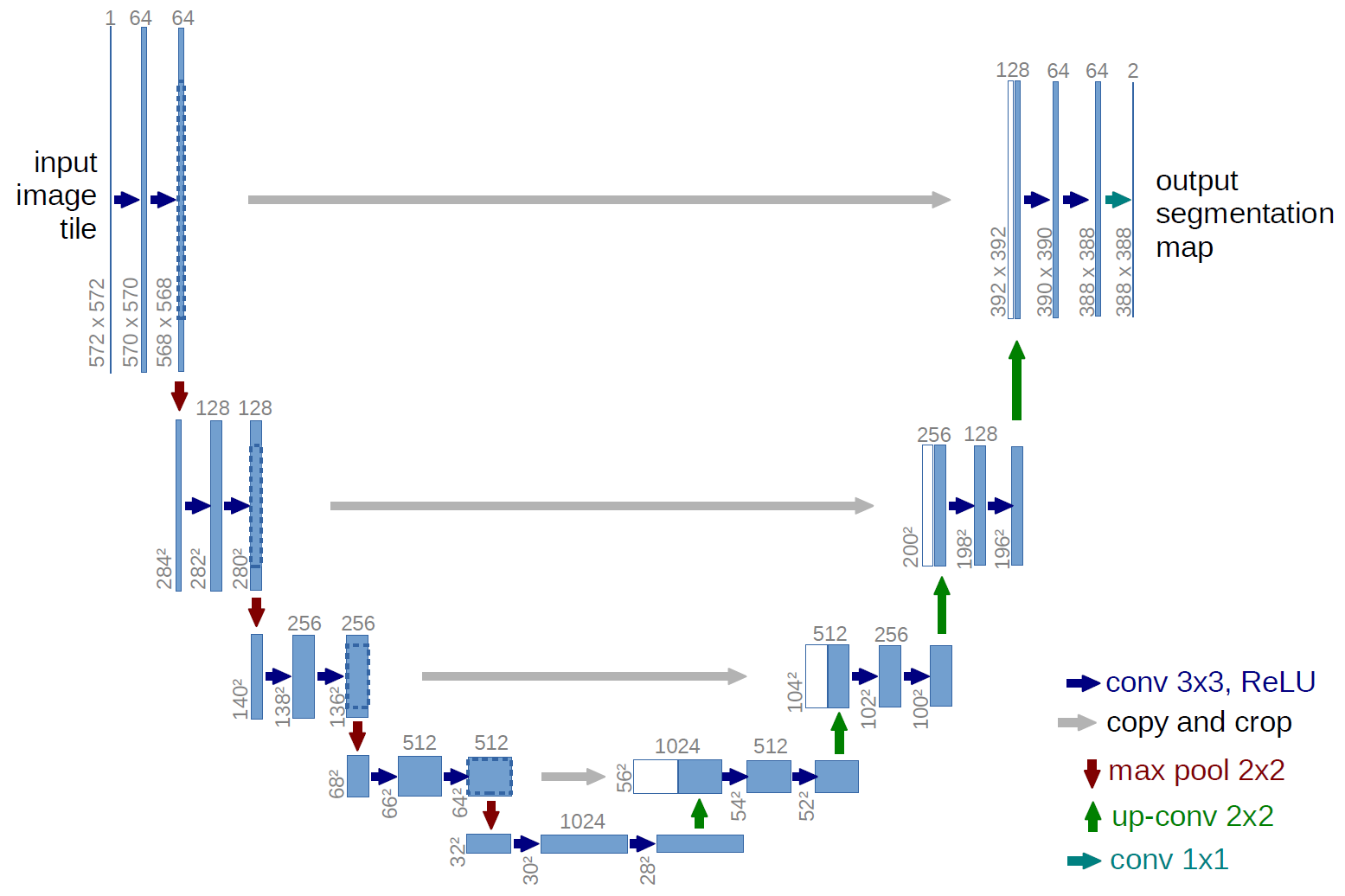
One method for helping CNNs preserve precise information from the original image is discussed in the UNET paper, which heavily inspired my architecture. UNET was originally designed for image segmentation, and so each pixel in a given input image is supposed be classified as one of N classes. In our case, we can adapt this approach so that our classes correspond to the 68 types of keypoints. Since our output will form a probability distribution over the pixels in our output image, we can get a concrete prediction by taking the expectation over the pixels of the model's output.
So how does UNET attempt to avoid the loss of spacial accuracy from pooling layers? The idea is as follows: we can follow our "down convolutions" (maxpools) with an equal number of "up convolutions", which will give our model a "U" shape. Then, we can forward information to the "up convolution" layers from their corresponding "down convolution" layer. Notably, this means that the final "up convolution" will have access to information from the input image that has not been pooled in any way. This idea is well captured in the following diagram taken from the linked UNET paper:
|
I tried various different sizes of network for my UNET implementation. Here is the final model that I used:
            LargeUnetCnn(
                (layer_down): MaxPool2d(kernel_size=2, stride=2, padding=0, dilation=1, ceil_mode=False)
                (layer1_down_across): Sequential(
                    (0): Conv2d(1, 64, kernel_size=(7, 7), stride=(1, 1), padding=same)
                    (1): LeakyReLU(negative_slope=0.01)
                    (2): Conv2d(64, 64, kernel_size=(5, 5), stride=(1, 1), padding=same)
                    (3): LeakyReLU(negative_slope=0.01)
                    (4): Conv2d(64, 64, kernel_size=(3, 3), stride=(1, 1), padding=same)
                    (5): LeakyReLU(negative_slope=0.01)
                    (6): Conv2d(64, 64, kernel_size=(3, 3), stride=(1, 1), padding=same)
                    (7): LeakyReLU(negative_slope=0.01)
                )
                (layer2_down_across): Sequential(
                    (0): Conv2d(64, 128, kernel_size=(3, 3), stride=(1, 1), padding=same)
                    (1): LeakyReLU(negative_slope=0.01)
                    (2): Conv2d(128, 128, kernel_size=(3, 3), stride=(1, 1), padding=same)
                    (3): LeakyReLU(negative_slope=0.01)
                    (4): Conv2d(128, 128, kernel_size=(3, 3), stride=(1, 1), padding=same)
                    (5): LeakyReLU(negative_slope=0.01)
                    (6): Conv2d(128, 128, kernel_size=(3, 3), stride=(1, 1), padding=same)
                    (7): LeakyReLU(negative_slope=0.01)
                )
                (layer3_down_across): Sequential(
                    (0): Conv2d(128, 256, kernel_size=(3, 3), stride=(1, 1), padding=same)
                    (1): LeakyReLU(negative_slope=0.01)
                    (2): Conv2d(256, 256, kernel_size=(3, 3), stride=(1, 1), padding=same)
                    (3): LeakyReLU(negative_slope=0.01)
                    (4): Conv2d(256, 256, kernel_size=(3, 3), stride=(1, 1), padding=same)
                    (5): LeakyReLU(negative_slope=0.01)
                    (6): Conv2d(256, 256, kernel_size=(3, 3), stride=(1, 1), padding=same)
                    (7): LeakyReLU(negative_slope=0.01)
                )
                (bottom_layer): Sequential(
                    (0): Conv2d(256, 512, kernel_size=(3, 3), stride=(1, 1), padding=same)
                    (1): LeakyReLU(negative_slope=0.01)
                    (2): Conv2d(512, 512, kernel_size=(3, 3), stride=(1, 1), padding=same)
                    (3): LeakyReLU(negative_slope=0.01)
                    (4): Conv2d(512, 512, kernel_size=(3, 3), stride=(1, 1), padding=same)
                    (5): LeakyReLU(negative_slope=0.01)
                    (6): Conv2d(512, 512, kernel_size=(3, 3), stride=(1, 1), padding=same)
                    (7): LeakyReLU(negative_slope=0.01)
                )
                (layer3_up): Sequential(
                    (0): ConvTranspose2d(512, 256, kernel_size=(2, 2), stride=(2, 2))
                )
                (layer3_up_across): Sequential(
                    (0): Conv2d(512, 256, kernel_size=(3, 3), stride=(1, 1), padding=same)
                    (1): LeakyReLU(negative_slope=0.01)
                    (2): Conv2d(256, 256, kernel_size=(3, 3), stride=(1, 1), padding=same)
                    (3): LeakyReLU(negative_slope=0.01)
                    (4): Conv2d(256, 256, kernel_size=(3, 3), stride=(1, 1), padding=same)
                    (5): LeakyReLU(negative_slope=0.01)
                    (6): Conv2d(256, 256, kernel_size=(3, 3), stride=(1, 1), padding=same)
                    (7): LeakyReLU(negative_slope=0.01)
                )
                (layer2_up): Sequential(
                    (0): ConvTranspose2d(256, 128, kernel_size=(2, 2), stride=(2, 2))
                )
                (layer2_up_across): Sequential(
                    (0): Conv2d(256, 128, kernel_size=(3, 3), stride=(1, 1), padding=same)
                    (1): LeakyReLU(negative_slope=0.01)
                    (2): Conv2d(128, 128, kernel_size=(3, 3), stride=(1, 1), padding=same)
                    (3): LeakyReLU(negative_slope=0.01)
                    (4): Conv2d(128, 128, kernel_size=(3, 3), stride=(1, 1), padding=same)
                    (5): LeakyReLU(negative_slope=0.01)
                    (6): Conv2d(128, 128, kernel_size=(3, 3), stride=(1, 1), padding=same)
                    (7): LeakyReLU(negative_slope=0.01)
                )
                (layer1_up): Sequential(
                    (0): ConvTranspose2d(128, 64, kernel_size=(2, 2), stride=(2, 2))
                )
                (layer1_up_across): Sequential(
                    (0): Conv2d(128, 64, kernel_size=(7, 7), stride=(1, 1), padding=same)
                    (1): Conv2d(64, 64, kernel_size=(3, 3), stride=(1, 1), padding=same)
                    (2): Conv2d(64, 64, kernel_size=(5, 5), stride=(1, 1), padding=same)
                    (3): Conv2d(64, 64, kernel_size=(3, 3), stride=(1, 1), padding=same)
                    (4): Conv2d(64, 64, kernel_size=(5, 5), stride=(1, 1), padding=same)
                )
                (final_layer): Sequential(
                    (0): Conv2d(64, 68, kernel_size=(1, 1), stride=(1, 1), padding=same)
                    (1): Flatten(start_dim=2, end_dim=-1)
                    (2): Softmax(dim=2)
                )
            )
Funnily enough, I actually tried using a much smaller UNET architecture before, but I was not satisfied with the final results. It turns out, however, that the reason why the final results were poor was actually because I was miscalculating the final pixel coordinates from the model's output (it was a slight error, and so the results were typically only off by a few pixels near the borders of the image). Because of this, I decided to try a larger architecture. While this larger model was training, I discovered the mistake in the pixel calculation and corrected it. However, because I had already put so much time into training the larger model I decided to just stick to it. Note however that the medium sized model performed almost as well as the large model, so it is fair to say that the size of this network is a bit overkill and similar results can be achieved at lesser cost.
Training
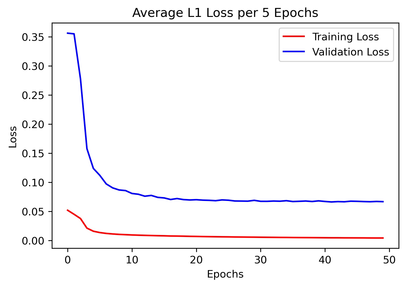
In parts 1-3, I used MSE as my loss function and didn't think too much of it. However in this part, I needed to write a custom loss function since my model outputs heatmaps, and I need to take the expected value of those heatmaps to get the corresponding pixel predictions. While doing this, I began to think about how effective MSE really is for our case. One property of MSE is that if a prediction is very close to the true label, the loss will be very low (even if it is not exactly equal). However, small inaccuracies get amplified when we convert the estimate of the pixel location in the downsampled image to a pixel location in the original image. Thus, we want to be as close to exact as possible. In order to accomplish this, I decided to try using L1 loss instead, which will penalize the model more for not matching labels exactly.
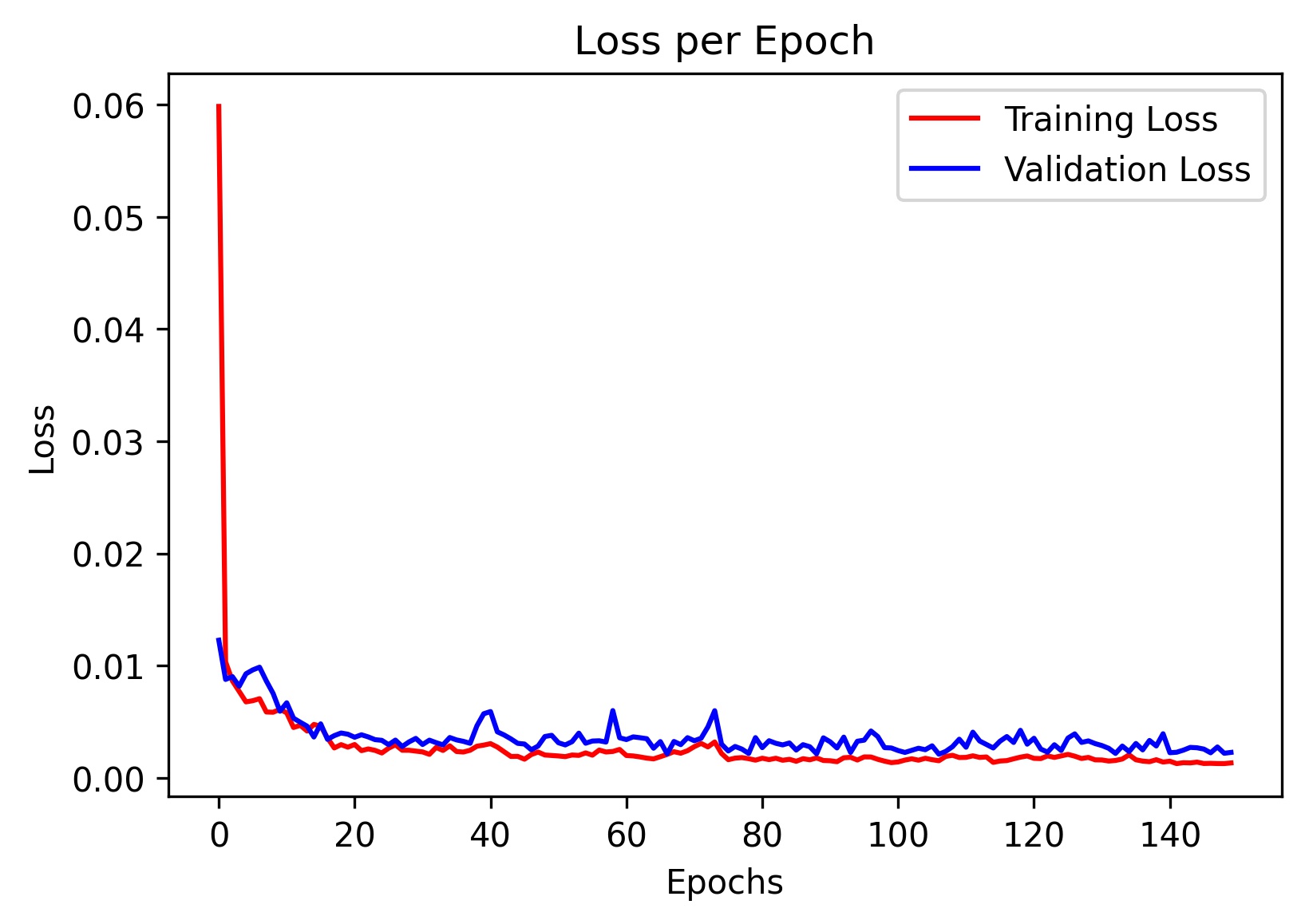
During training, I only recorded the training and validation loss every 5 epochs. Here is the loss curve for the final model I trained using the AdamW optimizer and a learning rate of 0.0001 (sorry that the x-axis ticks are messed up):
Note on Data Augmentation
In my opinion, the most important part to getting a good model is having really good data augmentation. At first, my data augmentation was rather lackluster and my model failed to generalize well. However, data augmentation allows us to pretend like our training set is much larger than it actually is. Some of the augmentations I used in this project are random rotations, random translations, random shears, and random brightness changes. However, the MOST important augmentation that I used was randomly changing the size of the bounding box.
From looking at the dataset, it is clear that the bounding boxes are not the best. Many of them are missing key parts of the face, and do not even contain all of the labeled keypoints. To fix this, I decided to increase the sizes of all the bounding boxes in the test set by about 10%. However, in order for the model to be able to classify these correctly, I needed to have data that had similar bounding boxes. Thus, I decided to add an augmentation to my data that would randomly increase the size of the provided bounding box between 0 and 20%. This ended up working amazing, as it taught the model to be resistant to variable backgrounds and support different precisions of bounding boxes.
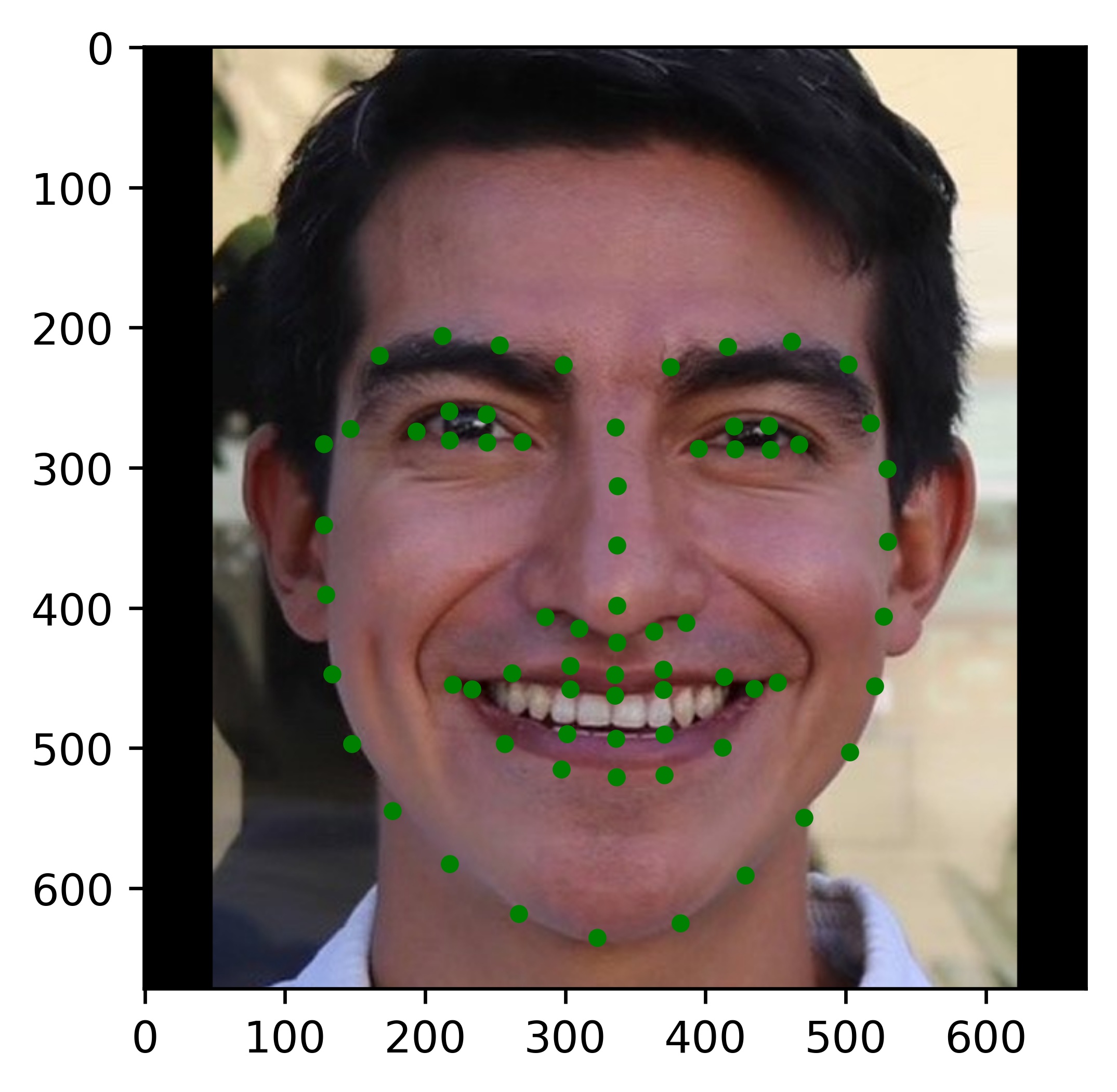
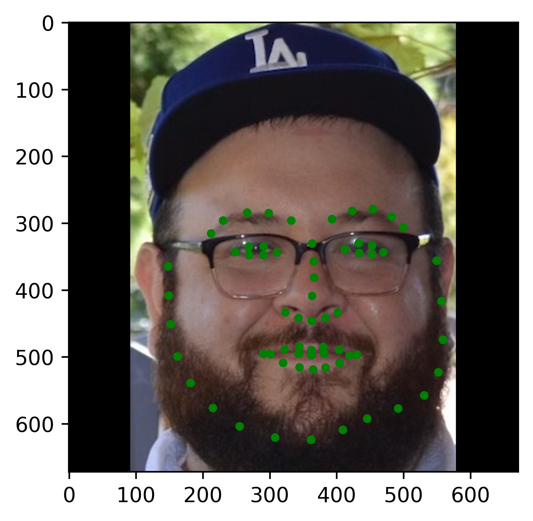
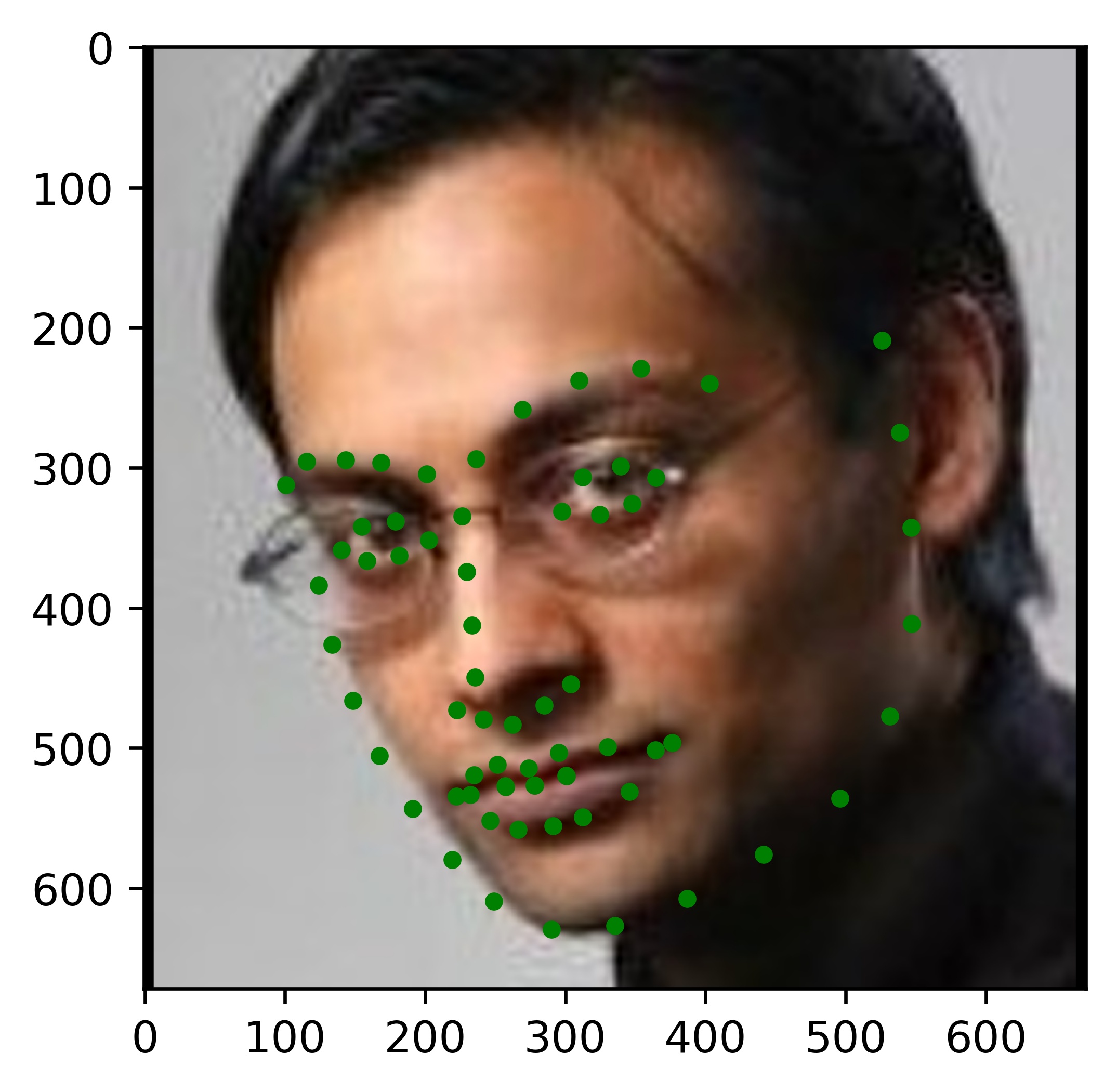
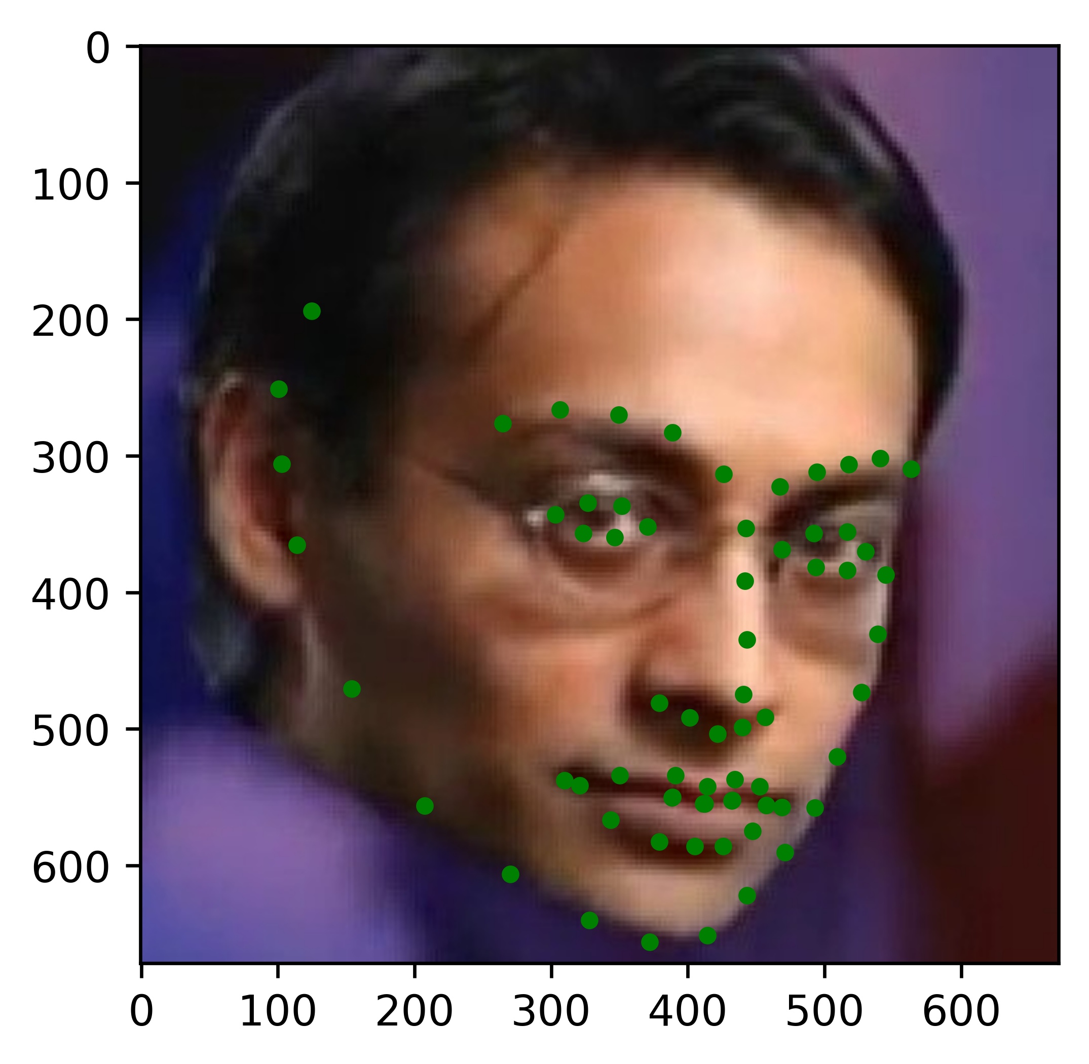
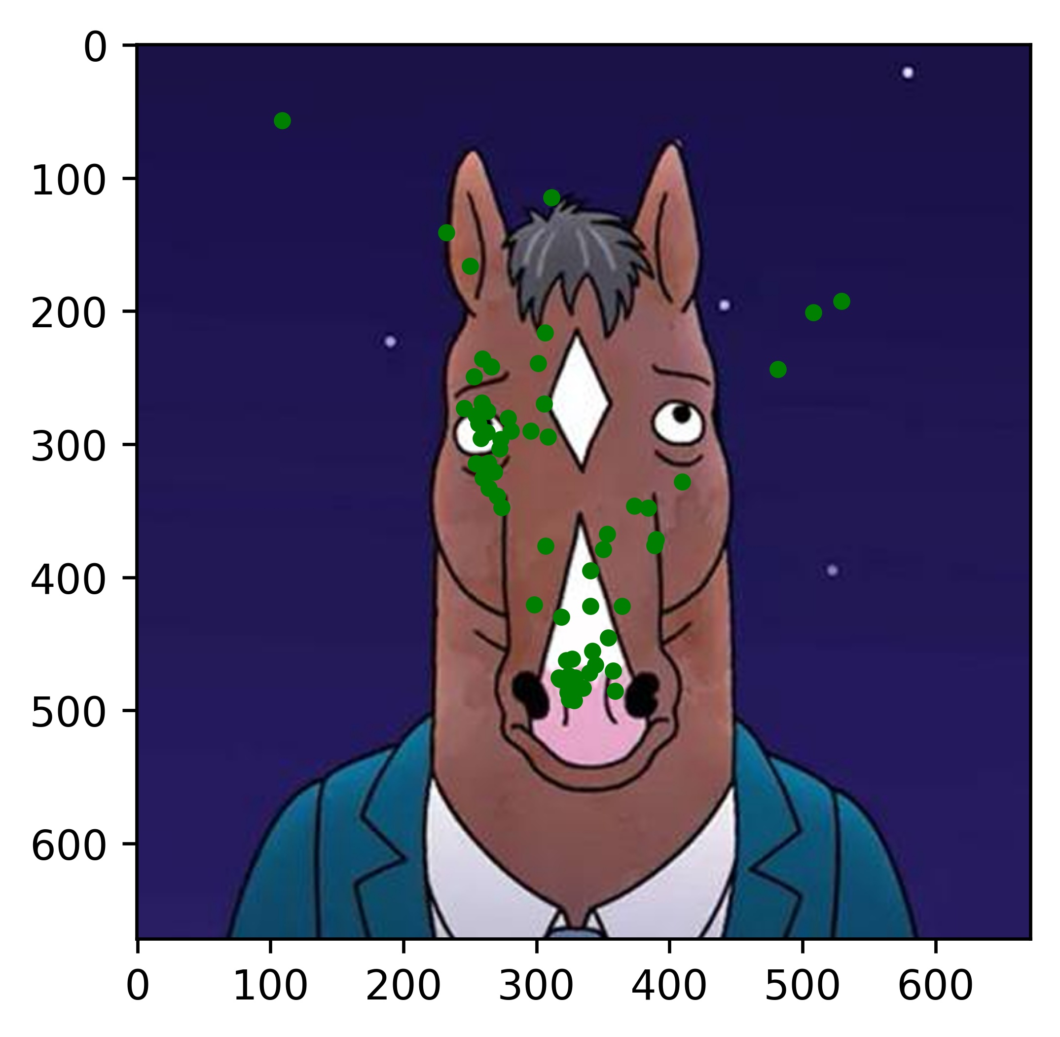
Results
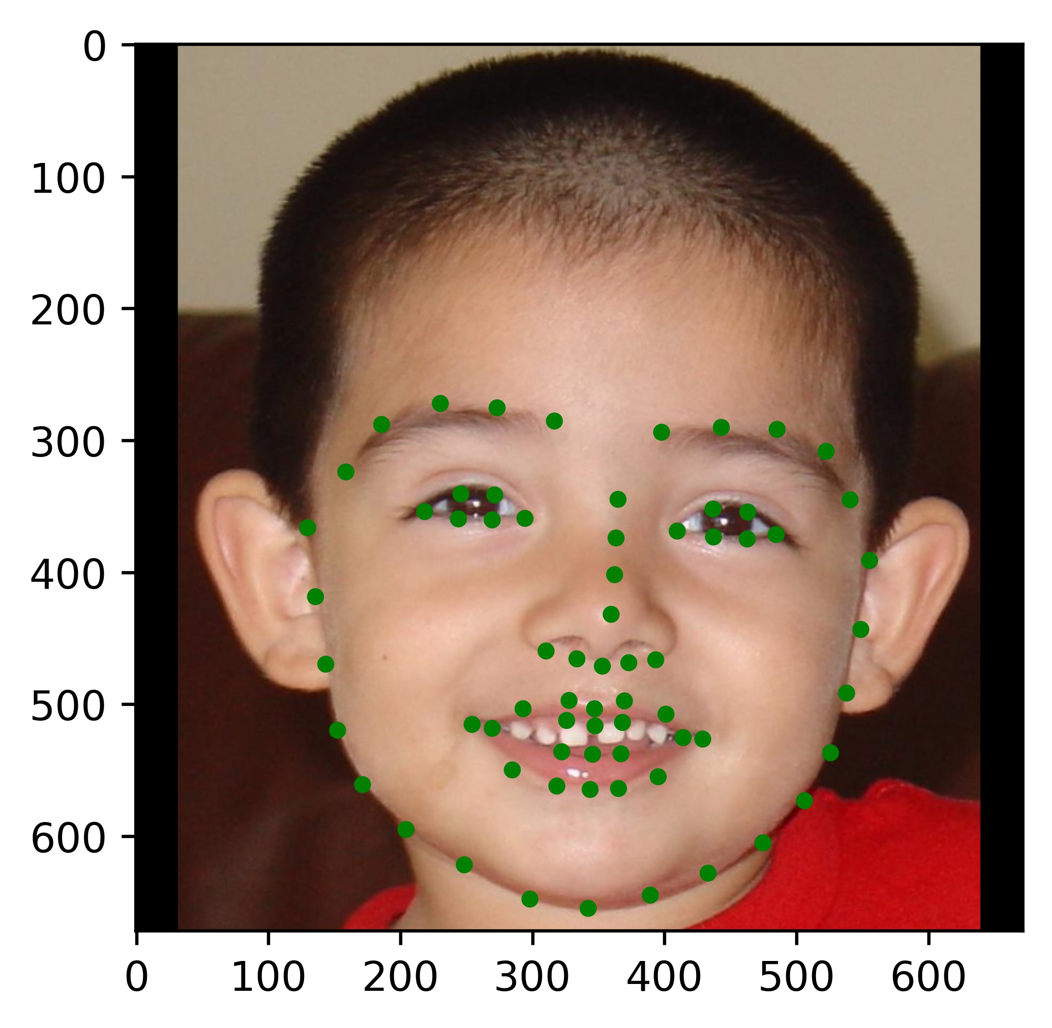
|
|
|
|
|
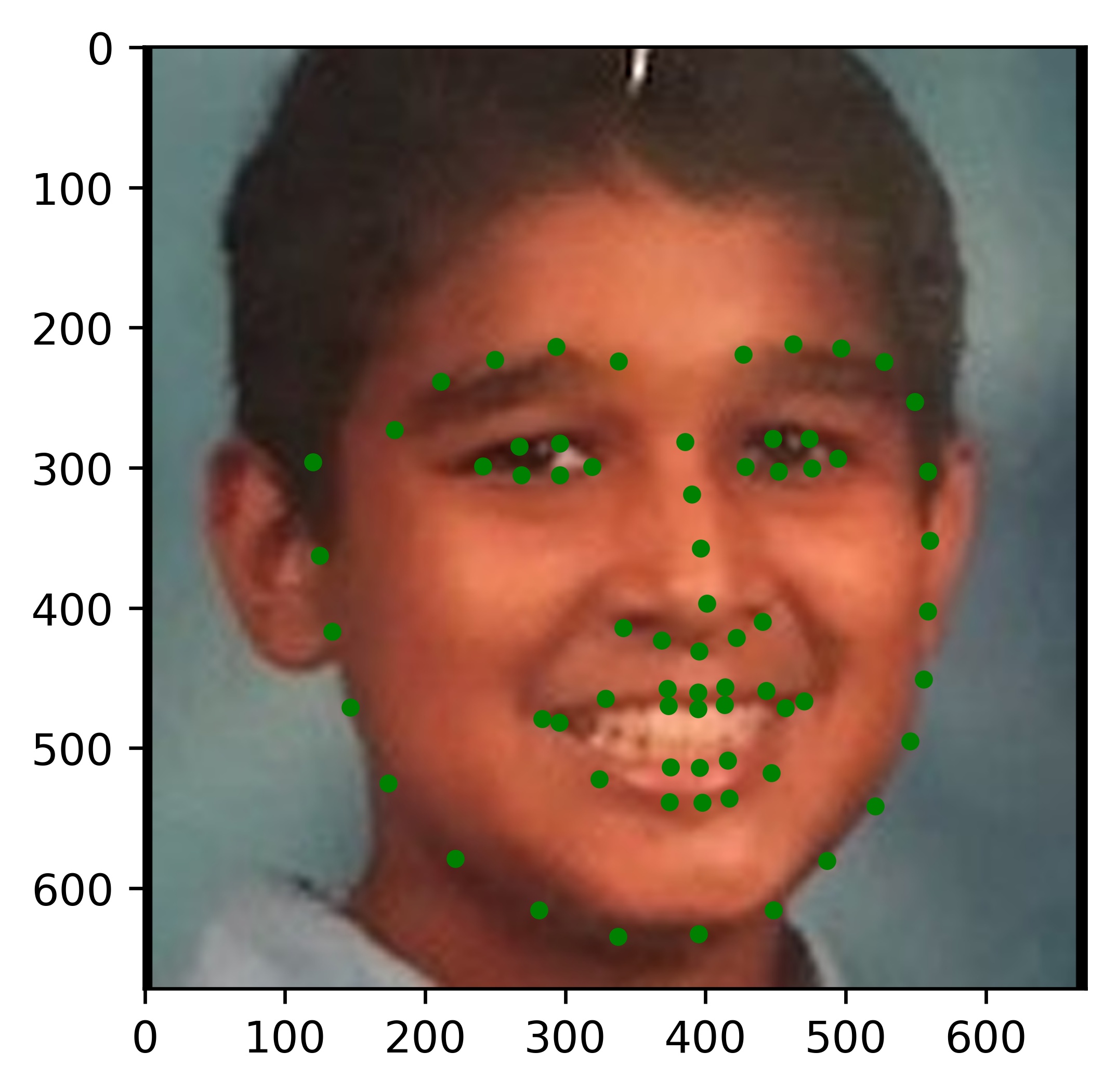
|
|
|

|
|
|
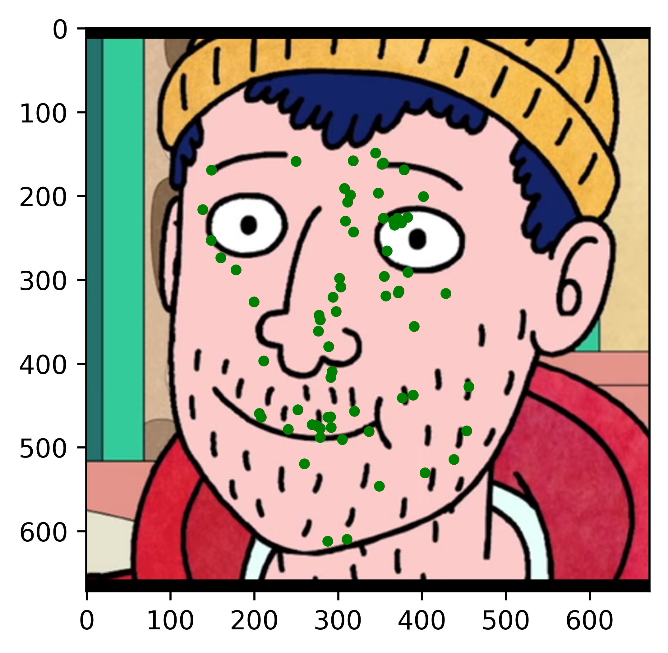
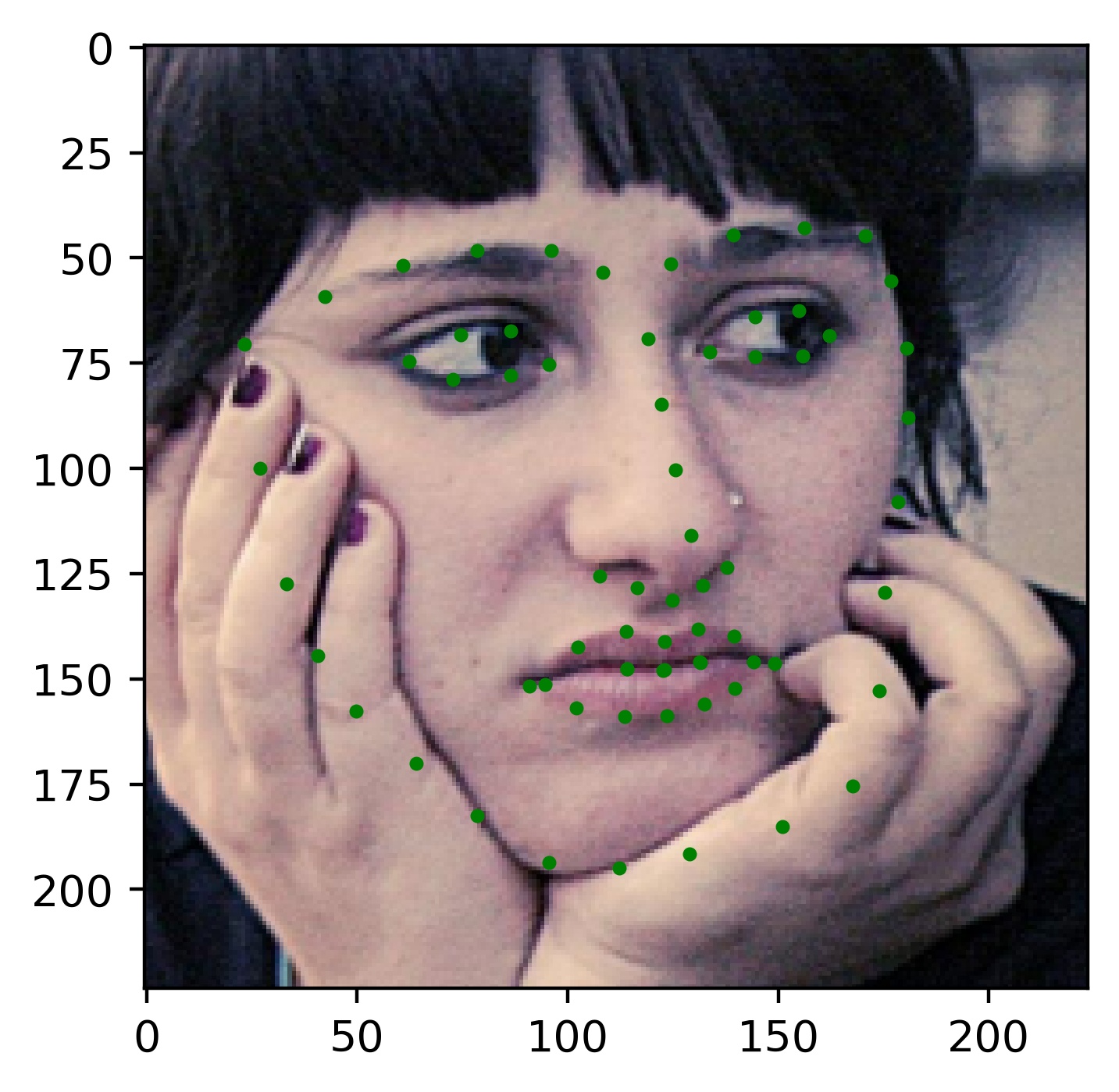
|
All the results on real faces came out really well! The cartoon faces did not work out so well, but perhaps we could fix this by incorporating some cartoon faces into the dataset. This would be an interesting continuation to this project. Another interesting task would be to write my own bounding box algorithm that is more well suited for this project.
Heatmaps
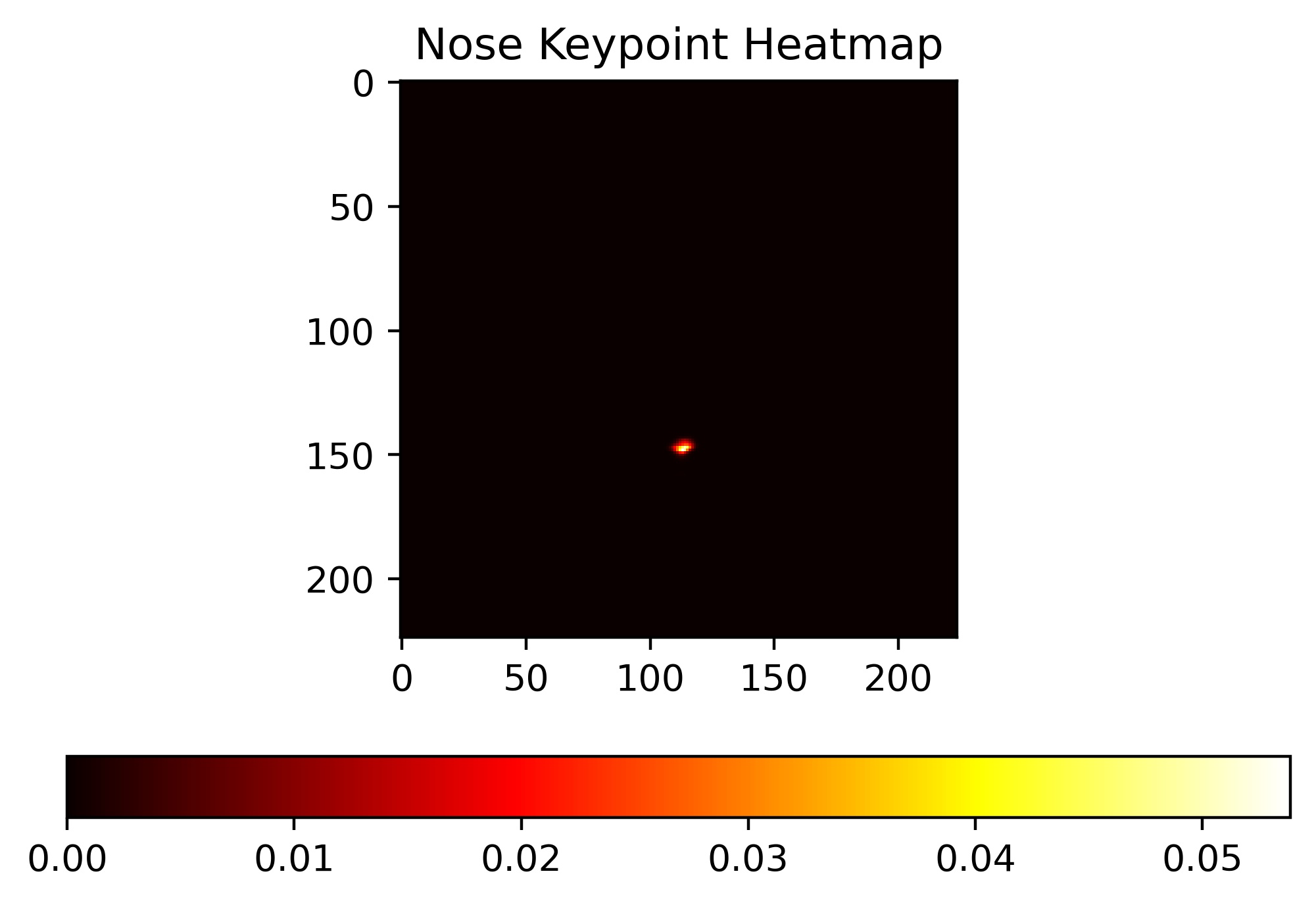
Since this architecture assigns a probability to each pixel, we can actually interpret the model's output as a heatmap. For example, we can look at the heatmap that corresponds to a pixel in the output image being a nose:
|
|
|
In this case, the model was extremely confident about classifying the tip of the nose, and so all of the probability mass is centered at the tip of the nose.
Follow Ups
I had a lot of fun doing this project and I learned a lot by experimenting with different approaches to this problem. Some things that I would like to try in the future related to this project are: