Arjun's CS294-26 Proj5
Part 1 Nose Tip Detection
As per the spec I downsampled the images to 80 x 60. I designed a CNN
with 3 convolutional layers with channels 12, 24, and 32 respectively. Each
I followed with max pooling and ReLU before feeding into a fully connected
classification network with a hidden dimension of 128. I trained the network
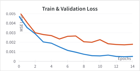
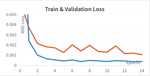
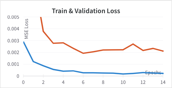
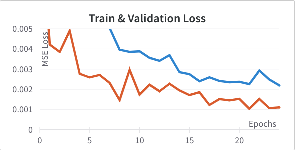
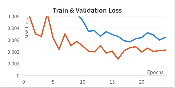
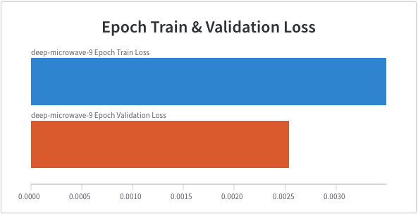
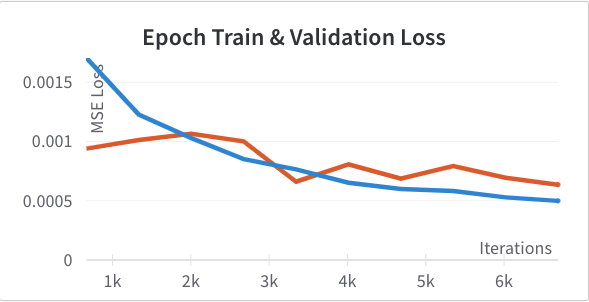
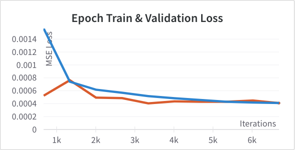
with Adam learning rate 1e-3 optimizing for mean squared error of the location of the nose tip. Below are the training and validation learning curves for this setup. In this and subsequent graphs the training loss is shown in blue and the validation loss in orange.
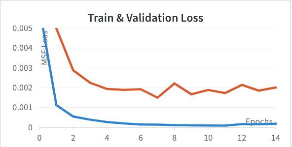
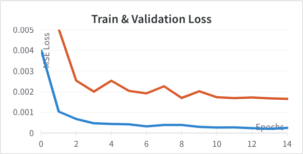
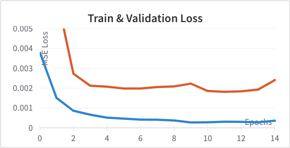
One thing I tried to improve the model was adding batch norm right after each
max pooling. Below are the loss curves after making this change. Training improves but validation doesn't change much we see signs of overfitting.
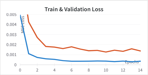
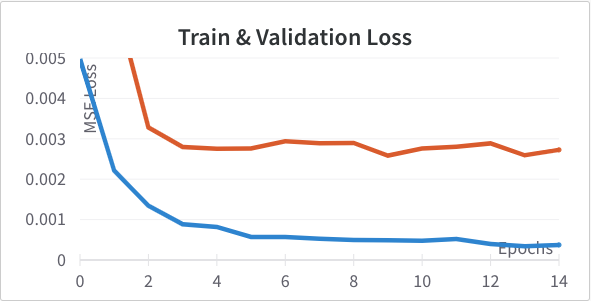
To help with regularization I tried added a dropout of 10% and 20% to the fully connected hidden layer to see if it helped the previous problem. 10% (Left) we actually see an improvement in validation loss; 20% (Right) was too much.
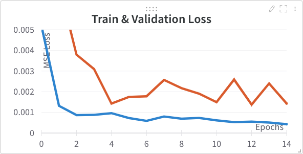
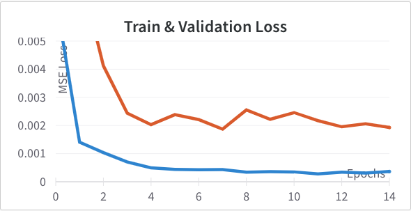
Here are the results for learning rate 3e-3 (Left) and 3e-4 (Right) instead of learning rate 1e-3. It turns out our problem can support a greater learning rate of 3e-3 without facing instability. 3e-4 is a little too slow and steady so we use 3e-3 moving forwards.
Next I tried adding an additional convolutional layer with 32 channels (Left) resulting in channels of [12, 24, 32, 32]. I also tried removing the final conv layer (Right) resulting in channels [12, 24]. Neither outperformed the original so I didn't incorporate either change.
Next I tried varying the size of the fully connected layer from it's baseline of 128 dimensions. I tried 256 (Left) and 64 (Right). Again, neither outperformed the original so I didn't incorporate either change.
I retrained for 50 epochs the best architecture was 3 convolutional layers (12, 24, 32 channels), using batch norm, then a fully connected layer with 128 units and dropout of 10%. Learning rate 3e-3 to train.
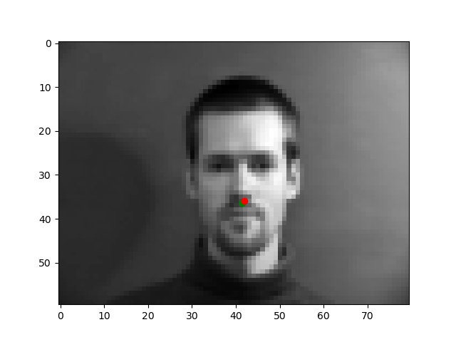
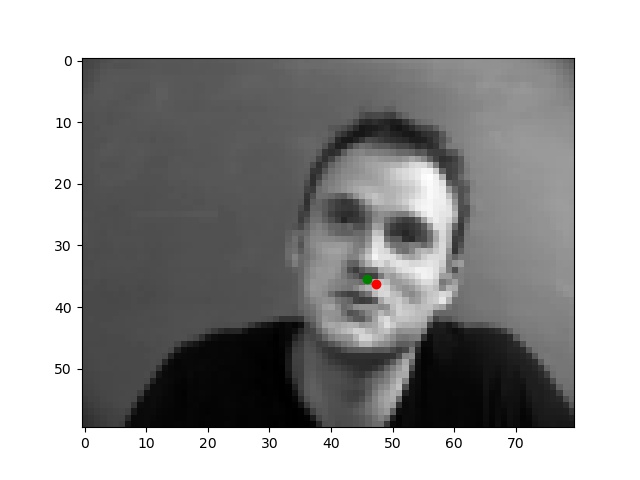
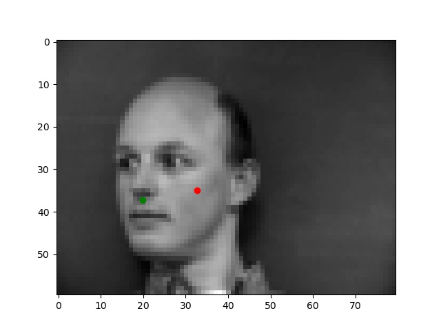
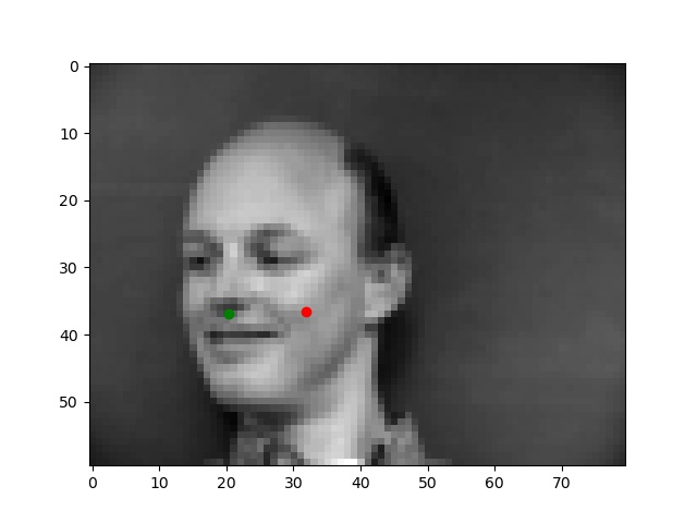
Below are the two images we do best on and the two we do worst on. Green dot is ground truth red dot is prediction. It's unsurprising that the two we do worst on are from the same person and orientation. I think the model might be confusing the texture of the cheek and how it's has a similar bump like a nose tip as well as how it's positioned where the nose often is. The ones we do best on are fairly typical shots which also makes sense.
Part 2 Full Keypoint Detection
We begin by training the best configuration from part 1 except now instead of predicting a 2D vector predicting a 116D vector which represents the 58 key points of interest on the face. We also apply data augmentation to help with the small size of our dataset with respect to the task we're trying to accomplish. I use a collor jitter as well as a random crop and resize. For the random crop and resize I make sure that the crop contains all 58 keypoints and maintains aspect ratio. Of course the keypoints themselves are adjusted after the fact. I don't apply data augmentation to the validation set to maintain integrity and stability of the dataset.Below are the loss curves for training with was the best configuration in Part 1.

Then I tried adding a convolutional layer with 64 channels. I also tried adding an additional fully connected layer with 128 dimensions (without the 64 channel conv layer) since representational capacity seems to be an issue. The results for the former (Left) and the latter (Right) below. The extra conv layer seemed to help but not the extra fully connected layer.
Given that there still seemed to be some room for capacity I tried doubling the size of the single fully connected layer from 128 to 256. Didn't improve performance.

I retrained for 100 epochs the best architecture was 4 convolutional layers (12, 24, 32, 64 channels), using batch norm, then a fully connected layer with 128 units and dropout of 10%. Learning rate 3e-3 to train.
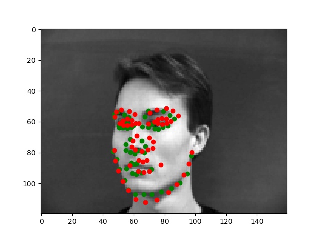
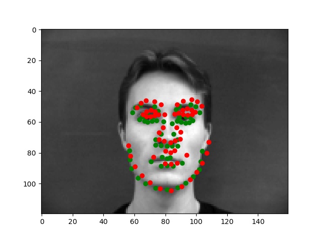
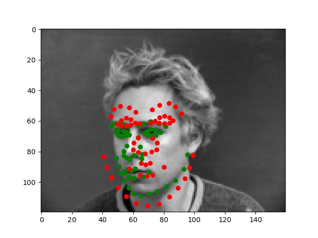
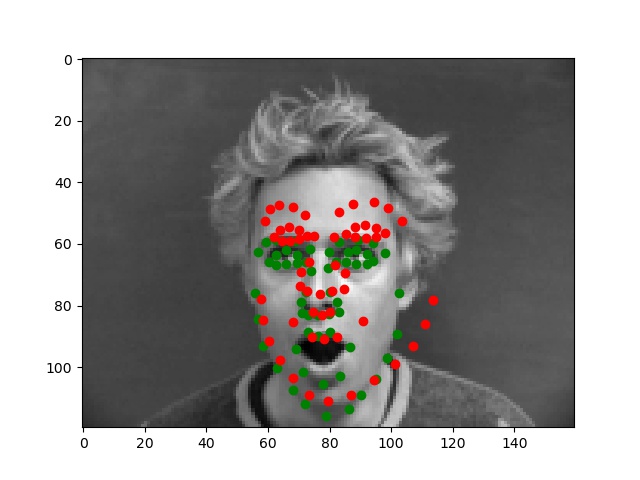
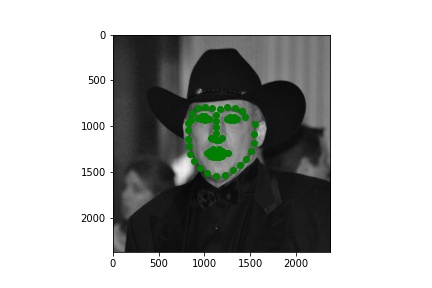
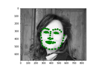
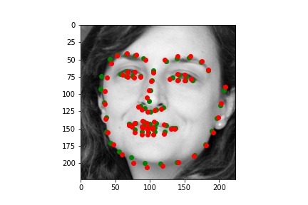
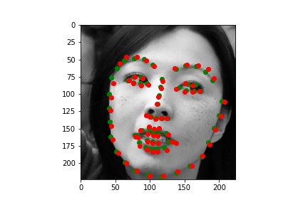
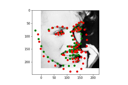
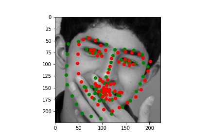
Below are the two images we do best on and the two we do worst on. Green dot is ground truth red dot is prediction. It's unsurprising that the two we do worst on are from the same person. I think it's because of the individuals hair making it seem like the face is a lot larger than it really is. The ones we do best on are fairly typical shots which also makes sense.
Part 3 Train with Larger Dataset
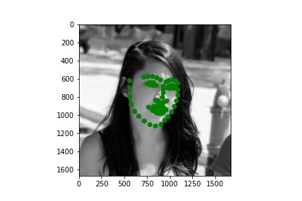
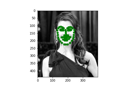
This dataset is definitely a lot more interesting due to it's increased volume and diversity. Here are a few sampled images with their ground truth keypoints.
I based my model on Resnet-18. I replaced the first convolutional layer which was originally expecting 3 channels for RGB with a a grayscale compliant single channel input. I replaced the output layer 512->1000 classes with 512->68*2 keypoints. I additionally do a post processing step of applying a 1.5 * sigmoid - 0.25. That is allow the model to provide a bounded output between (-0.25, 1.25) indicating the relative position (this is ultimately scaled up to the bounding box of the image). Regarding the images themselves I didn't simply provide what was in the bounding box because I noticed many times that cut of the chin or left out some keypoints. So I added padding of 0-25% in each of the 4 directions. The specific amount in each direction was our data augmentation along with a color jitter. For validation and testing I used constant padding of 12.5% on each side and no color jitter.
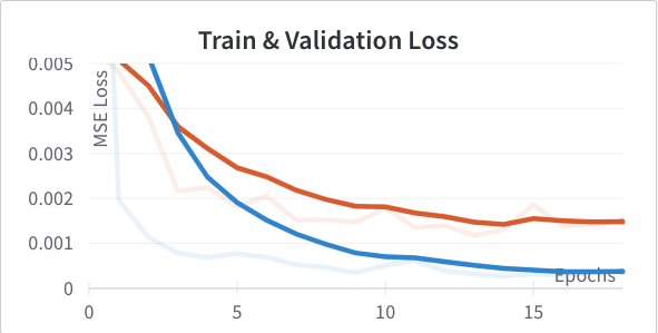
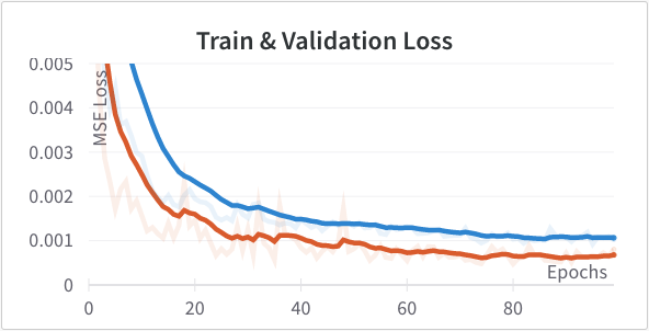
Regarding training, I include three graphs below. The first graph is the first epoch I ran to validate model saving. The second shows the next 10 epochs of proper training. This had an test mean absolute error of ~15.0 and started to show signs of overfitting. That's when I added the variable padding and scaled sigmoid and trained for another 10 epochs which is the final graph you see. Note the metrics are reported after the epoch is complete meaning we don't report the loss of a random model at the start which would probably be an order of magnitude or 2 higher. The final model on Kaggle had a test mean absolute error of ~7.7, not bad. For all of training I used batch size 10 and learning rate 3e-4.
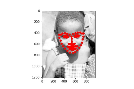
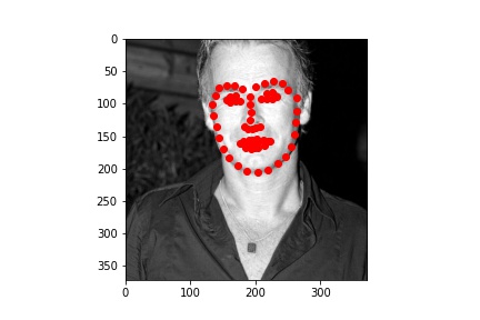
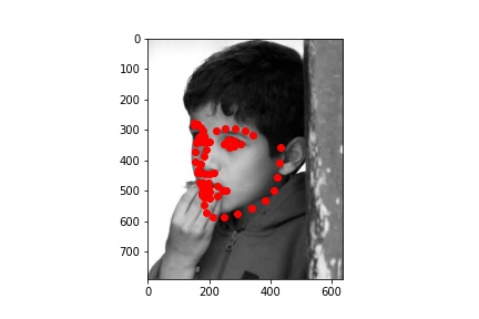
Here are the success and failure cases on the validation set. We find these by finding the worst 2 in a random set of 100 and the best 2 in the same set. This is pretty cool because unlike Part 2 with our simple model the deeper network seems to only be struggling with actually challenging images. The two failure cases here have the people with their hands obscuring their faces. On the other hand when the face is fully visibile the model is great.
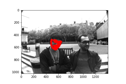
Finally here are some of the predictions on the test set projected on the whole original images. Pretty good on these random samples.