In this project, we learned how to implement convolutional neural networks with regression loss in order to train a model that would detect facial keypoints given an image of a person’s face. In the first part of the project, our neural network was small, consisting of 3 to 4 convolutional layers each with 12 to 32 channels. I created a model where the number of channels increased from one layer to the next. The convolutional layers were then followed by two fully connected layers and the task of this small neural network was to plot the nose tip keypoint on a given face. Due to its small size, the precision of the nose tip plotted by the model was not extremely accurate, doing better with faces that were looking more directly to the camera rather than profile pictures.
In the second part of the project, we used a similarly small neural network, though with a couple additional convolutional layers, in order to train a model that would output 58 keypoints of a given face. In this part we also implemented data augmentation methods such as random rotation of the image within the range [-15, 15] degrees, random translation within the range of [-10, 10] pixels and color jitter of the grayscale images affecting brightness and saturation. This neural network performed a bit better than in the first part, since it was larger and deeper, but still has a bit more difficulty accurately placing the keypoints on profile pictures.
In the third part of the project, we used the ResNet18 model which took a very long time to train. We also used a larger dataset of 6666 images in addition to applying data augmentation like in part 2. This neural network is a lot deeper and larger than the previous two parts and certainly performed better at facial keypoint detection due to its larger size. This project was very helpful for me to get acquainted with the methods of neural network training and also helped build some intuition for how hyperparameters like batch size, learning rate, kernel sizes, and the size and number of convolutional layers can either benefit or hurt a training model.
In this part, we used the 40 faces from the IMM Face Database, each face had six different picture poses taken. In total, there were 240 images in the database. As per the instructions, the first 32 of 40 faces were used for training the neural network, which is 192 images for training, and the last 8 of 40 faces were used for validating the neural network, which is 48 images for validation.
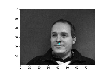
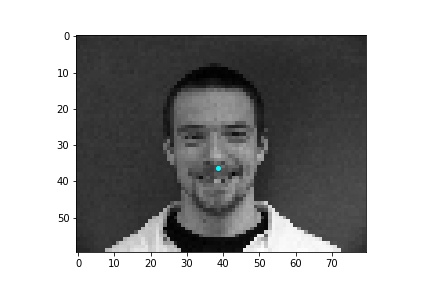
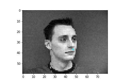
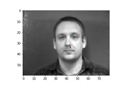
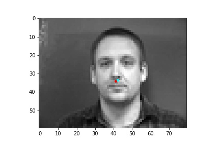
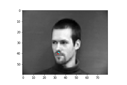
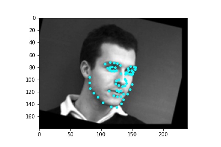
When creating the dataloader, mine expects an argument of whether the loaded data is used for training or validation. I thought it simpler to place the first 192 images in a subfolder labeled training and the last 48 images in a subfolder labeled testing so the dataloader could easily access the appropriate data when either building the training or validation dataloader. The loaded images are resized to 80x60 and converted to grayscale. Then the image pixel values are normalized to fall within the range -0.5 and 0.5 before the image is placed in a tensor and returned by the dataloader. Below are some sample images from the dataloader with the truth nose point plotted in cyan.
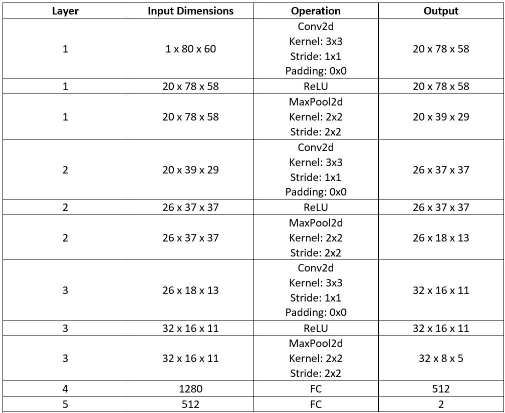
The neural network architecture I used for producing the result images was the following. The neural net only took in a single feature, since we are using a grayscale image as input, otherwise if we were to input a color image, then the number of input features to the neural network would be 3, one for each color channel. The image inputted into the neural network has dimensions 80x60 (width x height). Likewise, the number of output features that the neural network produces is 2, the x and y coordinates (normalized to be in the range 0 and 1) for the nose tip keypoint that the neural network predicted. I use three convolutional layers, the first of which outputs 20 channels, the second outputs 26 channels, and the third outputs 32 channels. Each convolutional layers uses a kernel size of 3x3 that is moved over the image with stride 1 in both the x and y directions and all three layers use 0 padding, so the image dimensions decrease by 2 in both the x and y direction after each convolutional layer. Following each convolutional layer, I apply the relu nonlinear activation function which is then followed by a maxpool with kernel size 2x2 and a stride of 2 in both the x and y directions. After the convolutional layers are done, I reshape the tensor so that it fits in the first fully connected layer which outputs 512 features and a relu is applied to this output. Then the second fully connected layer takes in the 512 features and outputs 2. No relu is used at this point and the neural network simply returns the 2 output values from this last fully connected layer as the approximation to the (x,y) position of the nose tip. I utilize a batch size of 2, a learning rate of 0.0001, and train for 20 epochs. Also, as per the instructions, I use the mean squared error loss MSELoss to compute the loss of each run and I train the neural network using Adam. Below is a table that better visualizes the layers of the neural network (batch size dimension excluded).
I use the model defined above and the 192 training images to train the neural network over 20 epochs. The plotted training and validation losses can be viewed below. It is observable that both the training and validation losses decrease as the number of epochs increases, which is to be expected since the weights in our neural network are being corrected to minimize output error. I do observe that even with a learning rate of 1e-4 the training loss drops relatively quickly within the first epoch and much more slowly afterwards. A smaller learning rate like 1e-5 will have a more gradual reduction in the loss for both the training and validation sets but the end loss after training does not justify the additional computation. Additionally, there is no observable point in the training where the validation loss increases while the training loss decreases (which suggests overfitting to the training data) so a learning rate of 1e-4 was selected.

And here is a zoomed in view of the training and validation losses after the first epoch of training was complete which better visualizes training and validation losses decreasing.

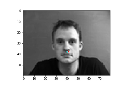
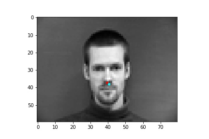
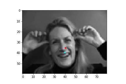
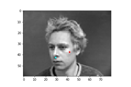
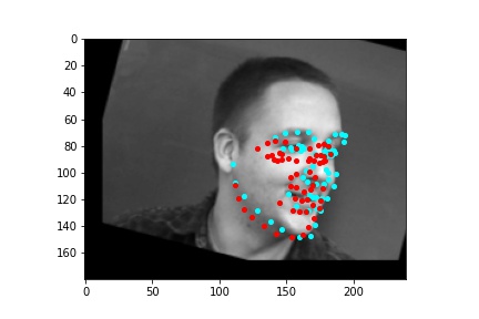
After training the neural network with the training set for the specified number of epochs, I set the neural network model into evaluation mode and fed the model the training and validation images. I then took the predicted nose point outputs for each image created by the model and plotted them on their respective image in red with the truth point, the one loaded from the dataset, in cyan like before. Below are some example images where the neural network produced pretty good results with respect to predicting the nose tip point.
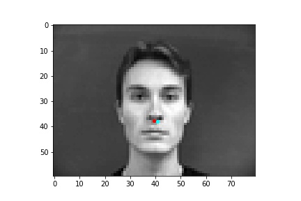
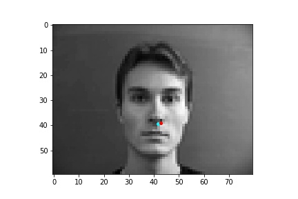
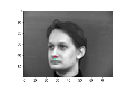
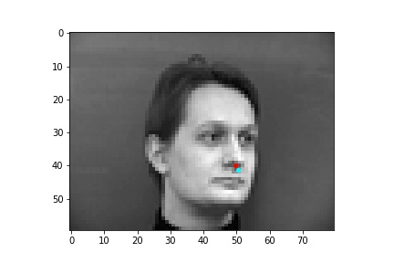
However, the neural network was not perfect and did produce predictions that were very much off from the truth value of the nose tip. Below are some examples where the neural network got the prediction wrong.
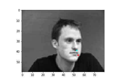
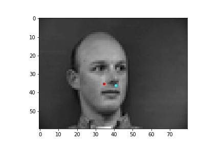
One potential reason why the neural network fails in these cases is because the people in the grayscale image are assuming different poses that move the nose keypoint further away from the anticipated location. I believe that the neural network is to some extend being influenced by the fact that it expects the nose keypoint to be within a certain region of the image frame rather than the possibility that it could be anywhere on the image. Following this idea, due to the limited amount of training data and lack of data augmentation in this part, the neural network learned really well where the nose tip was supposed to be when the person in the image was staring directly into the camera, but it becomes more difficult to extract facial features when the person has their head turned.
Varying number of layers: For this part, I attempted running 4 convolutional layers rather than 3 and noticed that it had a negative impact on my loss (increasing it). The additional kernels that needed to be trained probably required more epochs of training but it seemed as if the larger network on this data, just predicting a single keypoint, would result in overfitting quite easily as can be observed towards the last few epochs of training below. The validation loss began to flatten while the training loss continued to fall, which signaled to me that the network was beginning to overfit the training data. Additionally, there does not seem to be any additional, good information that the four-layer neural network can extract over the three layer one. This is likely due to the already small image size that we are inputting into the network, so the additional convolutional layer, not to mention additional maxpool that comes with the additional layer, is not helpful in extracting additional information from the image. After all, the output image size after the 3-layer convolutional network was 8x5 and with the 4th layer it was 3x2 so not much valuable information that can be extracted from that. This is why I decided to keep a three-layer convolutional network rather than four convolutional layers. Below are the loss curves when training the four-layer neural network:


Varying filter size: I did not observe any benefit to increasing the filter size at any level of the convolutional network. I tried 5x5 and 7x7 filters but the produced loss on both the validation and training datasets was not significantly improved. See the loss curves below for an example using a 7x7 filter for the first layer, a 5x5 filter for the second layer and 3x3 for the third layer. Again, this is likely due to the small size of the images to begin with. Also, with the larger filter sizes, I again observe the network starting to overfit the training data after the tend epoch, where the validation loss flattens out while the training loss continues to fall. Lowering the learning rate could potentially rectify this problem but given that the validation loss flattens where my selected neural network also reached, I doubt that a learning rate of 1e-5 would make a significant difference in the predictive power of the net.


Varying learning rate: I tried the following learning rates when training the model (1e-2, 1e-3, 1e-4, and 1e-5). When using a learning rate of 1e-2, the training became unstable. There was a lot of jitter on the loss and the network could not converge to a lower loss but instead was fluctuating at a higher loss. Obviously, this learning rate was too high and using an even larger learning rate would further exacerbate the thrashing observed when training the network, and potentially even result in the network increasing the loss over the training period. So I did not bother testing learning rates that were learning than 1e-2. A learning rate of 1e-3 was better, but not as good as 1e-4. I also testing 1e-5 though this learning rate was now becoming too small, requiring several more epochs of training before the network loss would decrease by a sizeable amount. This learning rate was too small and would require unnecessary computation for the loss to be reduced. Below are the loss curves for the tested learning rates. It is very apparent that learning rates of 1e-2 and 1e-3 are too large due to the jagged nature of both the train and validation loss curves, we want them to be fairly smooth and decreasing. The learning rate of 1e-5 is smoothly decreasing but is taking way too long and a learning rate of 1e-4 also provides a smooth decrease in loss but with less epochs required.


Varying batch size:: I also played around with different batch sizes and ultimately settled with a batch size of 2. A batch size of 1 took more time to train the model and also seemed to produce a slightly higher loss on the validation data. This may have been due to backpropagation correcting the network for each individual pose of a face which would result in overcorrecting the network to only learn that particular pose. So, I decided to try a larger batch size and see if on each iteration the network could learn from multiple poses at a time. The batch size of 2 did lower the loss on both the testing and validation sets by a bit and also offered a slight speed-up in training time. I also tried batch sizes of 3, 4, and 6, but the more I increased the batch size, the worse the neural network performed on the validation set and in the case of a batch size of 6, the loss was more than double my loss with a batch size of 2.
In this part, we used the 40 faces from the IMM Face Database, each face had six different picture poses taken. In total, there were 240 images in the database. As per the instructions, the first 32 of 40 faces were used for training the neural network, which is 192 base images for training, and the last 8 of 40 faces were used for validating the neural network, which is 48 images for validation. The two main differences from the last part are that first, we are now training the neural network to predict all 58 keypoints on the face and second, we apply data augmentation each time the image is loaded and sent to the net which is explained a bit more in the next section.
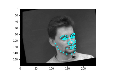
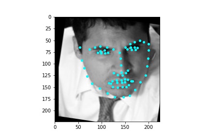
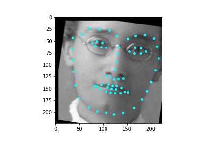
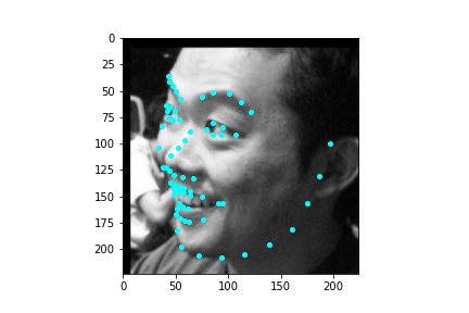
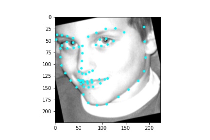
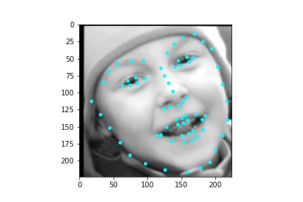
Again, when creating the dataloader, mine expects an argument of whether the loaded data is used for training or validation. I thought it simpler to place the first 192 images in a subfolder labeled training and the last 48 images in a subfolder labeled testing so the dataloader could easily access the appropriate data when either building the training or validation dataloader. The loaded images are first augmented in a random way. I apply a random color jitter which randomly changes the brightness and saturation of the image. I then also apply a random rotation on the image which is sampled from within the range -15 to 15 degrees inclusive and also apply a random translation shift on the image which is sampled from -10 to 10 pixels inclusive. The same transformations applied to the image are also applied to the keypoints. The image is then converted to grayscale and the image is resized to 240x180. Then the image pixel values are normalized to fall within the range -0.5 and 0.5 before the image is placed in a tensor and returned by the dataloader. Below are some sample images from the dataloader with the truth keypoints plotted in cyan.
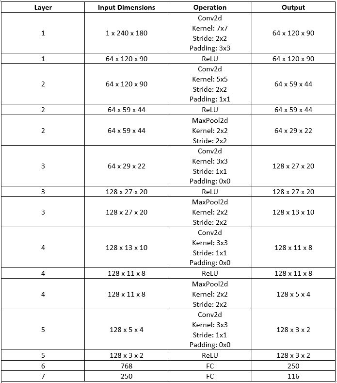
The neural network architecture I used for producing the result images was the following. The neural network only took in a single feature, since we are using a grayscale image as input, otherwise if we were to input a color image, then the number of input features to the neural network would be 23, one for each color channel. The image inputted into the neural network has dimensions 240x180 (width x height). Likewise, the number of output features that the neural network produces is 116, the x and y coordinates (normalized to be in the range 0 and 1) for the 58 facial keypoints predicted by the neural network. I use five convolutional layers, the first of which outputs 64 channels, the second outputs 64 channels, the third outputs 128 channels, the fourth outputs 128 channels, and the fifth outputs 128 channels. The first convolutional layer uses a kernel size of 7x7, which is moved over the image with stride 2 in both the x and y directions, and utilizes a padding of 3 pixels around the image. The second convolutional layer uses a kernel size of 5x5, which is moved over the image with stride 2 in both the x and y directions, and utilizes a padding of 1 pixel around the image. The third, fourth, and fifth convolutional layers utilize a kernel size of 3x3, which is moved over the image with stride 1 in both the x and y directions, and do not add any padding around the image. Following each convolutional layer, I apply the relu nonlinear activation function. The maxpooling function is not applied after every convolutional layer, only after the second, third, and fourth convolutions (the first and fifth convolutions are not followed by a maxpool function). The maxpool function is initialized with a kernel size of 2x2 and a stride of 2 in both the x and y directions. After the convolutional layers are done, I reshape the tensor so that it fits in the first fully connected layer which outputs 250 features and a relu is applied to this output. Then the second fully connected layer takes in the 250 features and outputs 116. No relu is used at this point and the neural network simply returns the 116 output values from this last fully connected layer as the approximations to the (x,y) positions for the 58 facial keypoints. I utilize a batch size of 2, a learning rate of 0.00001, and train for 15 epochs. Also, as per the instructions, I use the mean squared error loss MSELoss to compute the loss of each run, though in this part I initialize the loss function with a reduction of ‘sum’ which is why the loss values on the Y axis of the loss curves graph are in a different scale than the other two parts. I also train the neural network using Adam. Below is a table that better visualizes the layers of the neural network (batch size dimension excluded).
I use the model defined above and the 192 training images (which are augmented with random rotation, translation, and color jitter every time they are loaded by the dataloader) to train the neural network over 15 epochs. The plotted training and validation losses can be viewed below. It is observable that both the training and validation losses decrease as the number of epochs increases, which is to be expected since the weights in our neural network are being corrected to minimize output error. I had to do quite a bit of experimentation to get the loss curves to decrease smoothly since the smaller models I had tested (convolution channels between 12 and 24) would either not converge or would overfit on the training data and produce an extremely jagged loss curve for the validation loss. This is how I ultimately settled on making my network much bigger, after all we now have to predict 58 keypoints on a much larger input image than in part 1. The smaller learning rate of 1e-5 and a batch size of 2 seemed to produce the best results in terms of preventing overfitting while keeping the neural net learning by decreasing the loss in both the training and validation sets. Additionally, in the loss curve below, there is no observable point in the training where the validation loss increases significantly while the training loss decreases which is an indication that the model was not overfitting to the training data.

And here is a zoomed in view of the training and validation losses after the first epoch of training was completed which better visualizes the training and validation loss decreasing.

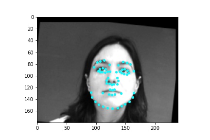
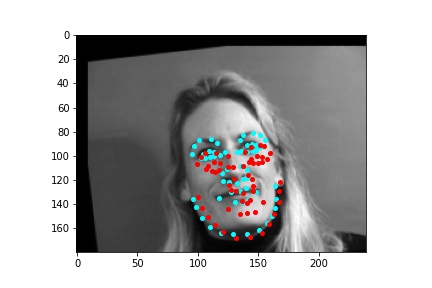
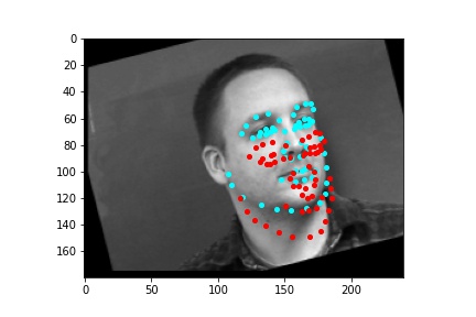
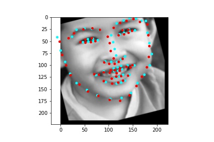
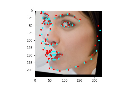
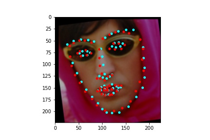
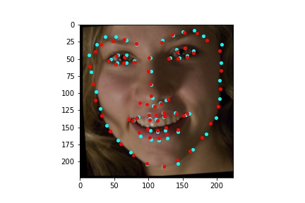
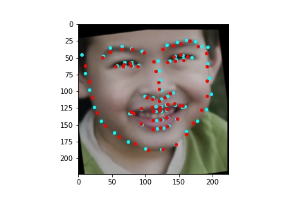
After training the neural network with the training set for the specified number of epochs, I set the neural network model into evaluation mode and fed the model the training and validation images. I then took the predicted keypoint outputs for each image created by the model and plotted them on their respective image in red with the truth point, the one loaded from the dataset, in cyan like before. Below are some example images where the neural network produced pretty good results with respect to predicting the facial keypoints.
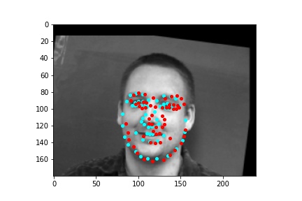
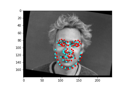
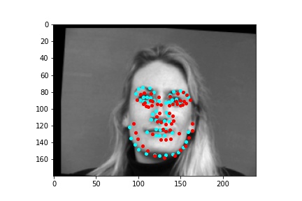
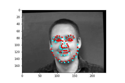
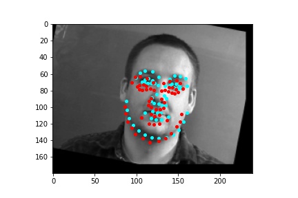
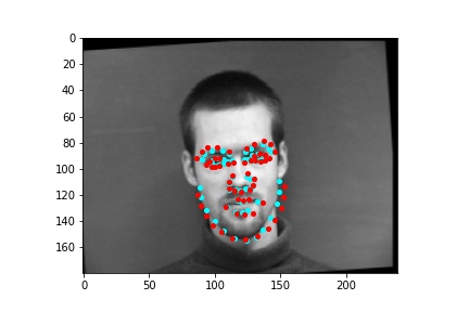
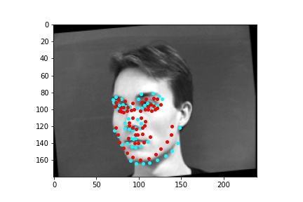
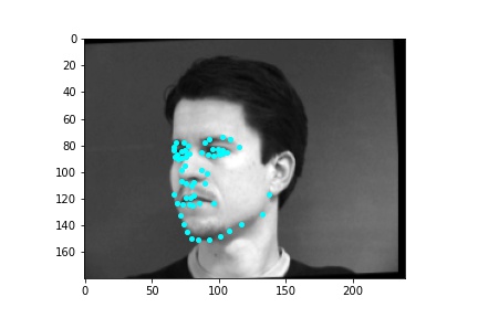
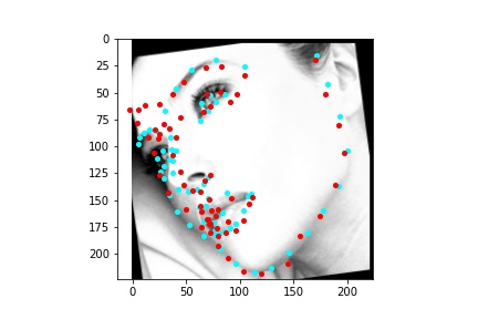
However, the neural network was not perfect and did produce predictions that were very much off from the truth values of the facial keypoints. Below are some examples where the neural network got the prediction wrong.
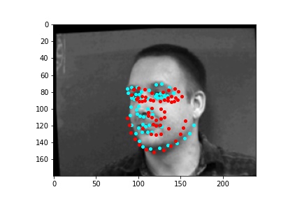
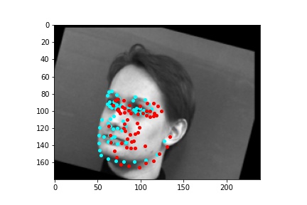
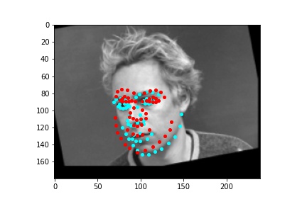
Like in part 1, I observe that the neural network struggles more with identifying keypoints on faces that are not looking directly into the camera. Again, this may be due to the limited amount of data available even with the data augmentation methods being applied. It can also be that the network is not large enough yet to accurately identify the profiles of faces and predict facial keypoints for them.
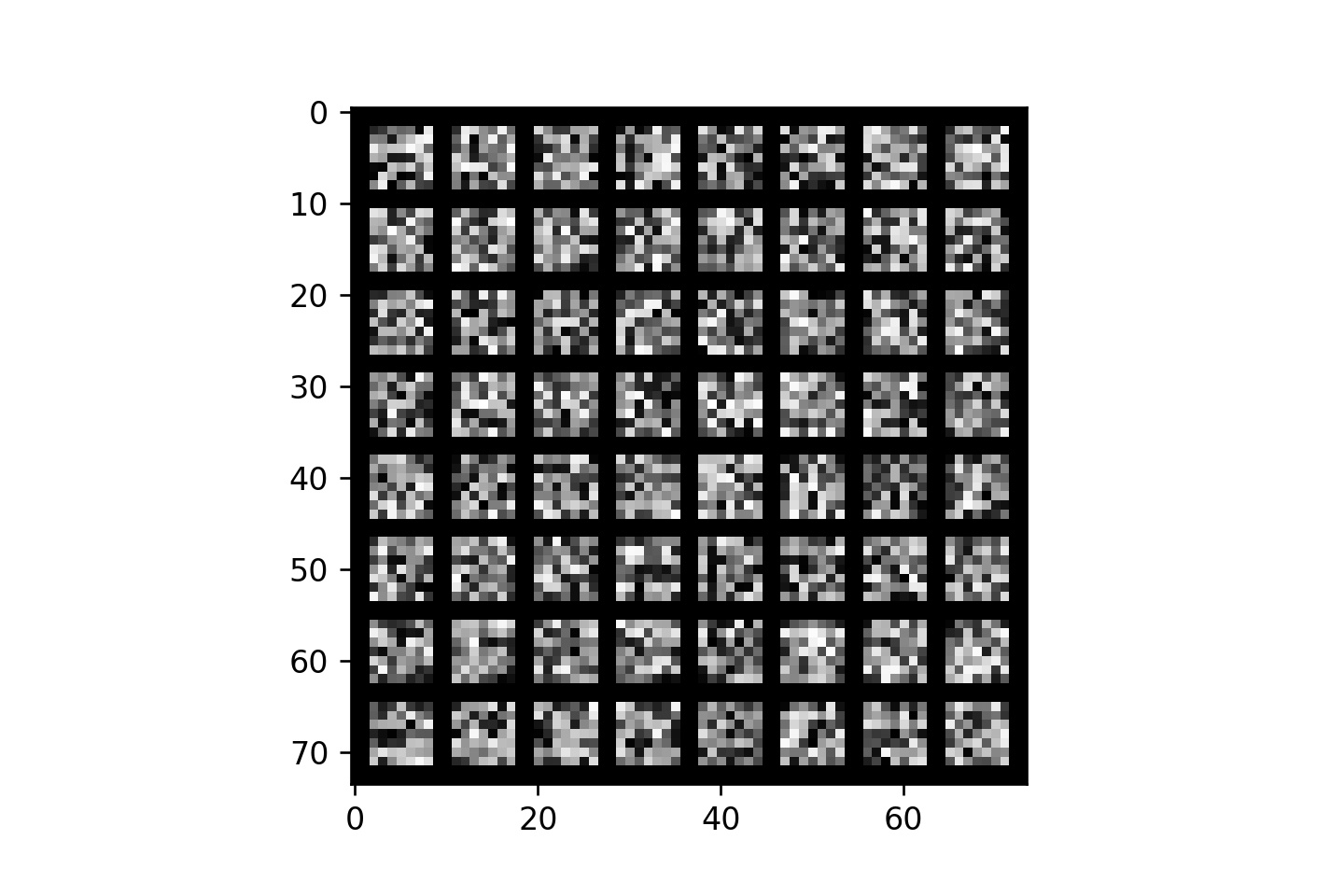
The network I trained is relatively large, even though a bigger network may still be required to more accurately predict facial keypoints. Due to the size of my network, I only plot the learned filters in the first convolution, which consist of 64 7x7 filter kernels. I normalize the values of these kernels to be between 0 and 1 so that they can be shown below in grayscale.
In this part, we use the ibug face in the wild dataset to train our neural network for facial keypoint detection. For training, this database consists of 6666 images which I divide roughly as 80% for training and 20% for validation. Additionally, this dataset consists of 68 facial keypoints, which means that our neural network will have to output 136 features from its last fully connected layer corresponding to the (x,y) position for each of the 68 facial keypoints. We are told to train using ResNet18 for this part which I do but I also experiment with some other neural networks like ResNet50, inputting color images rather than grayscale to the neural network, and using SmoothL1Loss instead of MSELoss.
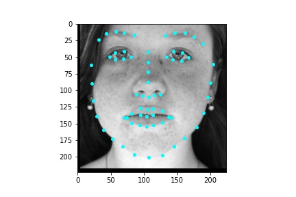
When I created this dataloader, it also accepts an argument of whether we are constructing a train dataset or a validation dataset, but depending on what argument is passed-in it utilizes different images from the database to construct the dataset. The datasets constructed contain roughly 80% of the training images in the train dataset and 20% of the training images in the validation dataset. The training images are defined in the train xml file which was provided with the dataset. Each image that is returned by the dataloader is first preprocessed to only crop the face within the frame. I did notice that using the square bounding box provided in the xml file would frequently result in facial features being plotted outside of the cropped image frame. I solve this issue by first assessing the furthest feature points corresponding to that image and then enlarging the square bounding box by a certain amount as to reduce the number of features that will fall outside of the cropped image frame. Of course the bounding box is used to crop the image and then the image is resized to 224x224. Afterwards, the same data augmentation steps are applied where a random color jitter affecting brightness and saturation are applied to the color image, then the image is converted to grayscale, a random rotation is applied within the range -15 to 15 degrees inclusive and random translation is applied within the range -10 to 10 pixels inclusive. The pixel values of the grayscale image are normalized to fall within the range -0.5 and 0.5 before the image is placed in a tensor and returned by the dataloader. The corresponding facial keypoints undergo the same transformations so that they align with the returned image. Below are some sample images from the dataloader with the truth keypoints plotted in cyan.
The neural network architecture I used for producing the result images was the following. The neural network I use is the standard ResNet18 model that is available from the models package in torchvision. I modified this model so that the first convolution only took in a single feature, since we are using a grayscale image as input, otherwise if we were to input a color image then no modification would need to be made to the first convolution. The image inputted into the neural network has dimensions 224x224 (width x height). Likewise, the number of output features that the neural network needs to produce is 136, the x and y coordinates (normalized to be in the range 0 and 1) for the 68 facial keypoints predicted by the neural network. Thus, I also had to modify the last fully connected layer to only output 136 features rather than the 1000 classification features it normally has. The ResNet18 neural net is quite lengthy so instead of listing out every single step in the ResNet18 neural net in a table like I have previously done, I will overview its general architecture and why it is called a residual net. ResNet18 begins by applying a convolution with a 7x7 kernel, a stride of 2, and padding of 3 pixels around the image. Afterwards, a batch norm is performed, a ReLU follows, and a maxpool is then applied with a kernel size of 3x3, a stride of 2 and a padding of 1 pixel around the image. This part can be thought of as the pre-processing step for the ResNet architecture and is the same across all ResNet variations. Now we begin applying the layers. There are four convolutional layers each of which contain two blocks of convolutions. Each block really applies two total convolutions so each layer contains four convolutions and since there are four layers, that is a total of 16 convolutions, not including the first one performed in the pre-processing step. The first layer performs convolutions that output 64 features and use 3x3 kernels. The second layer performs convolutions that output 128 features and use 3x3 kernels. The third layer performs convolutions that output 256 features and use 3x3 kernels and the fourth layer performs convolutions that output 512 features and use 3x3 kernels. Within each layer, after the first basic block, there is a connection from a previous layer that, when needed, is sampled using a convolution with a 1x1 kernel to create the same number of output features as the current layer. This connection to the previous layer allows the neural net to learn from both its current state and a previous state and significantly improves the robustness of the model. Being able to look at information in previous layers is also why the neural net is called a residual net. For training I utilize a batch size of 16, a learning rate of 0.00001, and train for 30 epochs. Also, I use the mean squared error loss MSELoss to compute the loss of each run. I also train the neural network using Adam.
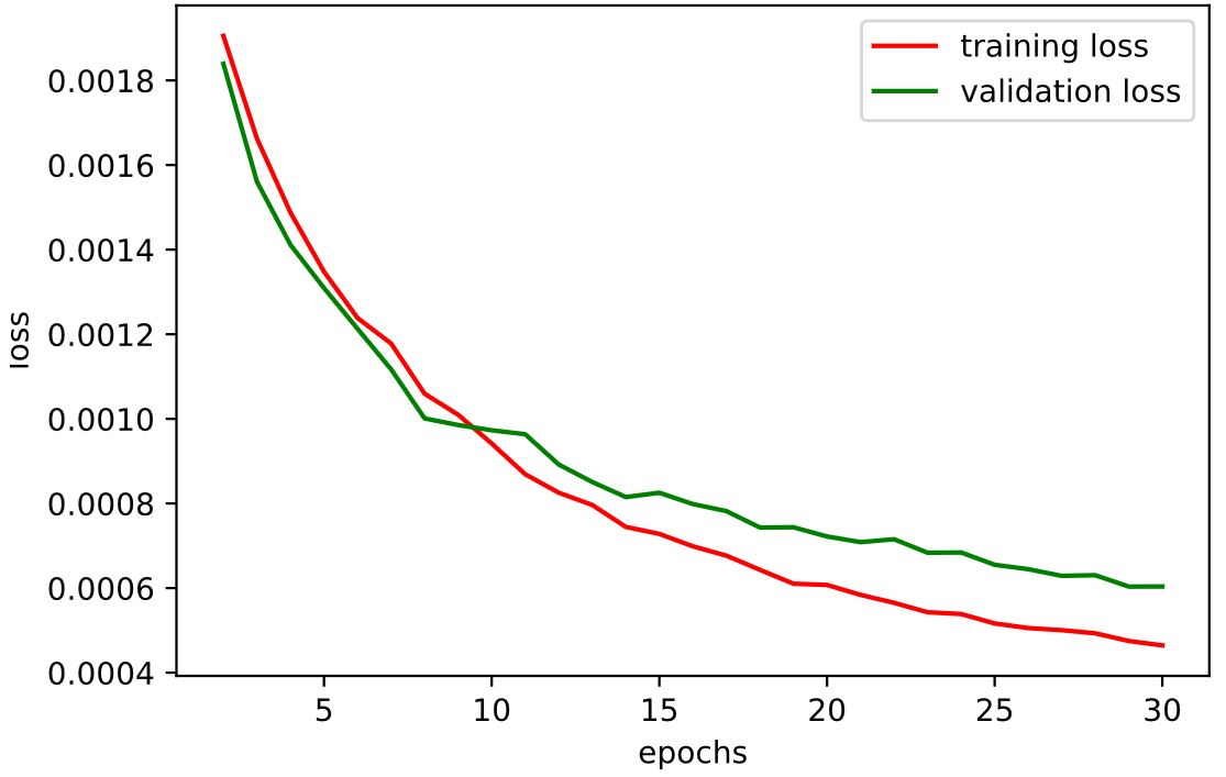
I use the model defined above and approximately 80% of the images defined in the train xml file to perform training of the neural network. Again, the images returned by the dataloader are augmented with random rotation, translation, and color jitter every time they are loaded. The plotted training and validation losses over the 30 epochs of training can be viewed below. It is observable that both the training and validation losses generally decrease as the number of epochs increases, which is to be expected since the weights in our neural network are being corrected to minimize output error. After some testing, I settled on smaller learning rates for the ResNet model since the larger model benefited from more granular corrections when training over a large number of epochs. That is why for this run I ultimately settled on using a learning rate of 1e-5 and the batch size of 16 also performed better than my original testing with a batch size of 256 or 64.
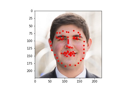
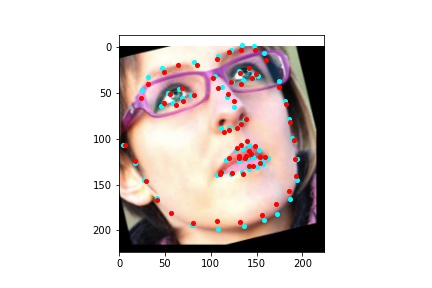
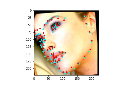
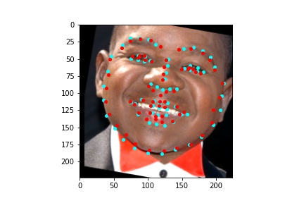
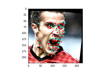
After training the neural network with the training set for the specified number of epochs, I set the neural network model into evaluation mode and fed the model the training and validation images. I then took the predicted keypoint outputs for each image created by the model and plotted them on their respective image in red with the truth point, the one loaded from the dataset, in cyan like before. Below are some example images where the neural network produced pretty good results with respect to predicting the facial keypoints.

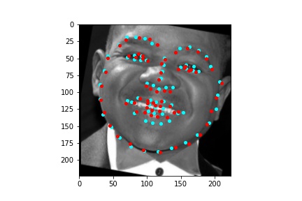
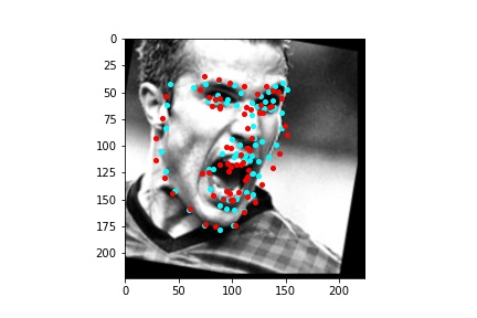
The above model, which utilized the standard ResNet18 neural net with a modified first convolution to accept grayscale images and a modified final fully connected layer to output 136 features performed relatively well as can be visualized with the above images, though some of them had keypoints slightly off such as the man who seems like he is screaming. When I submitted the predicted keypoints for the test set to Kaggle, I was assessed a score of 11.82192
I also tried training a larger neural network, in this case the standard ResNet50. For this neural network, I also decided to not input grayscale images into the net but rather the color images. I did run into the problem where some of the training images were already grayscale so in my loader, I check the dimensionality of the image and then convert grayscale images into grayscale (color) images so that they are of the right dimensions to be processed by the network. These were few images and I could have just discarded them but I do believe there was something to still be learned from those images which the neural net could extract. The first convolution layer of the ResNet50 neural net is the same as ResNet18, applying a convolution with a 7x7 kernel, a stride of 2, and padding of 3 pixels around the image. Afterwards, a batch norm is performed, a ReLU follows, and a maxpool is then applied with a kernel size of 3x3, a stride of 2 and a padding of 1 pixel around the image. Again, this part can be thought of as the pre-processing step for the ResNet architecture and is the same across all ResNet variations. Now is the point where the differences begin. Resnet50 also has four convolutional layers but within each layer, there are more than just two blocks of convolutions. In the first layer, there are three blocks of convolutions, the second layer has four, the third layer has six blocks of convolutions, and the fourth layer has three blocks of convolutions. Within each block, three convolutions are applied, which also differs from ResNet18. The kernel sizes and feature outputs of the convolutions within each layer are also different. Within each block, the first and third convolution always use a 1x1 kernel while the second convolution uses a 3x3 kernel. Additionally, only the first and second convolutions output the same number of features, the third convolution outputs four times as many outputs as the first and second convolutions. Meanwhile, the first convolution of the batch in the following layer outputs twice the features of the first and second convolutions in each batch of the previous layer. For example, the first layer consists of three blocks with convolution feature outputs (64, 64, and 256). Then the second layer consists of four blocks with convolution feature outputs (128, 128, and 512). After all the layers are finished, we enter the fully connected network which I modified to output 136 features for the predicted facial feature coordinates. Again, because it is a residual network, within each layer, after the first basic block, there is a connection from a previous layer that, when needed, is sampled using a convolution with a 1x1 kernel to create the same number of output features as the current layer. This connection to the previous layer allows the neural net to learn from both its current state and a previous state and significantly improves the robustness of the model. Being able to look at information in previous layers is also why the neural net is called a residual net. For training I utilize a batch size of 16, a learning rate of 0.00001, and train for 30 epochs. Also, I use the SmoothL1Loss to compute the loss of each run (I found that this loss function performed slightly better on color image inputs than MSELoss). I also train the neural network using Adam.
I use the model defined above and approximately 80% of the images defined in the train xml file to perform training of the neural network. Again, the images returned by the dataloader are augmented with random rotation, translation, and color jitter every time they are loaded. The plotted training and validation losses over the 30 epochs of training can be viewed below. It is observable that both the training and validation losses generally decrease as the number of epochs increases, which is to be expected since the weights in our neural network are being corrected to minimize output error. After some testing, I settled on smaller learning rates for the ResNet model since the larger model benefited from more granular corrections when training over a large number of epochs. That is why for this run I ultimately settled on using a learning rate of 1e-5 and the batch size of 16 also performed better than my original testing with a batch size of 256 or 64.

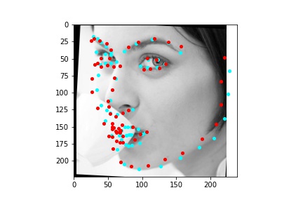
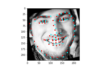
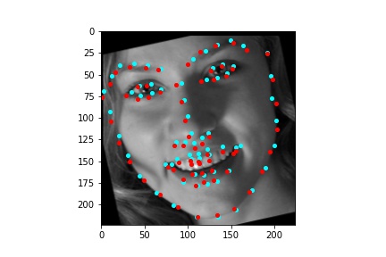
After training the neural network with the training set for the specified number of epochs, I set the neural network model into evaluation mode and fed the model the training and validation images. I then took the predicted keypoint outputs for each image created by the model and plotted them on their respective image in red with the truth point, the one loaded from the dataset, in cyan like before. Below are some example images where the neural network produced pretty good results with respect to predicting the facial keypoints.
The above model, which utilized the standard ResNet50 neural net with a modified final fully connected layer to output 136 features performed relatively well as can be visualized with the above images, and also seems to have done better than ResNet18 at predicting facial keypoints. When I submitted the predicted keypoints for the test set to Kaggle, I was assessed a score of 9.49675
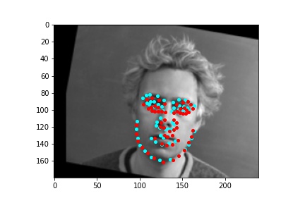
Since the ResNet50 neural net performed better at learning where facial keypoints belong on the image, I utilized it to generate facial keypoints on five images which I found (one of which is me). The input images and the output results are viewable below.
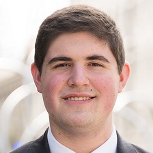
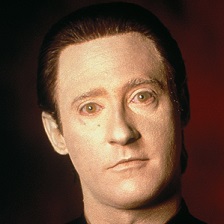
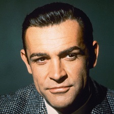
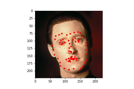
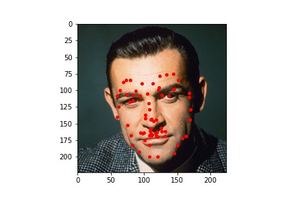


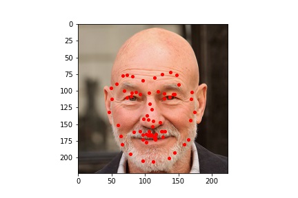
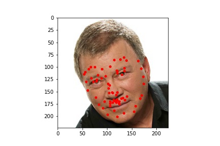
Here we can see that the neural network was not perfect but overall did a very good job at identifying the facial keypoints. We can see though with these pictures that the neural network is a bit sensitive to forehead wrinkles, which is why I think some of the top keypoints are placed a bit higher than they should be. I was also surprised by how well the network handled beards.
This project was at times very frustrating but also very fun. Training neural networks certainly is an art and I started to get the hand of how to interpret the validation and training loss curves so that I could modify my hyperparameters or the model architecture appropriately. I also learned the underlying process by which modern computer vision is implemented and I was a bit amused as to how long it takes to train a big neural network, and then it very quickly predicts feature keypoints once the model has been trained.