CS 194-26 Fall 2021 - Project 5
Facial Keypoint Detection with Neural Networks
George Gikas
Part 1: Nose Tip Detection
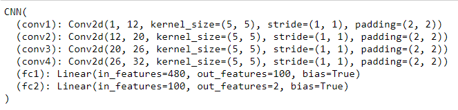
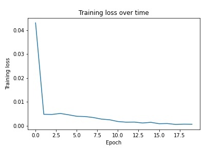
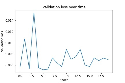
For the first part, I implemented nose tip detection by creating a neural net with 4 convolutional layers ranging from 12-32 output channels followed by two fully connected layers that produced two values, the x and y coordinates of the nose tip. When running the net, I used learning rates 0.0001, 0.001, and 0.01. I found that the first one led to extremely fast overfitting while the third one learned quite slowly, so I used the middle learning rate to fix this. I ran the neural net for 20 epochs with a learning rate of 0.001. Below is the architecture of the neural net as well as the training and validation loss graphs:
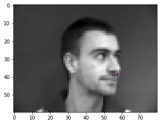
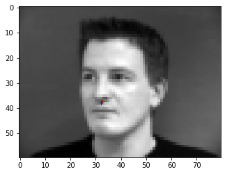
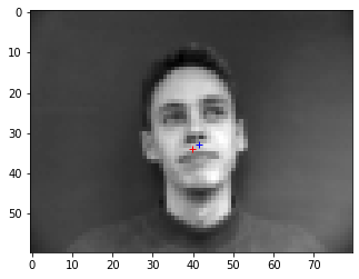
I then selected four images and their outputs to examine, two of which held good results and two of which missed the nose tip. I believe that the reason the net was unable to determine the nose tip in these images was because of the lighting of the face, and how it would be more difficult to pick a location. In the below images, the blue point is the ground truth and the red point is the predicted value:
 Good example #1
|
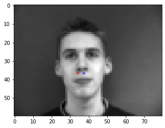
 Good example #2
|
 Bad example #1
|
 Bad example #2
|
Part 2: Full Facial Keypoints Detection
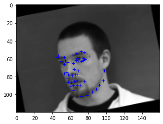
For this part, I implemented rotation of the image and points as a method of data augmentation. I also implemented shifting, but found my validation scores to do better without the shifting. Below are a couple of images sampled from the dataloader, with the ground truth points plotted:
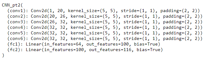
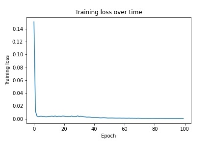
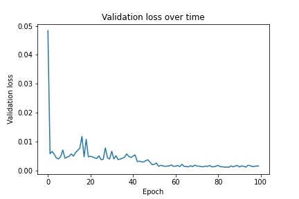
I then implemented a neural net with 6 convolutional layers ranging from 12-32 channels as well as two fully connected layers that distill the parameters down to x,y coordinates for each of the 58 points (58x2). I used a learning rate of 0.001 and ran for 100 epochs. Below is the architecture of the net as well as graphs of the training/validation loss:
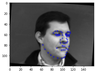
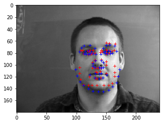
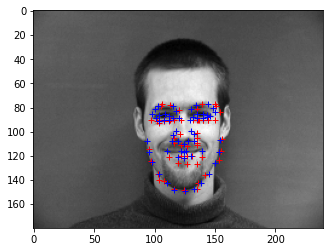
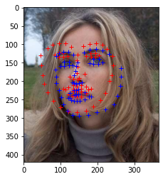
Below are four images that I selected to examine. The neural net was able to produce satisfactory coordinates for two of the images, while it struggled on the other two. If I had to take a guess as to why the other two images may have done more poorly, it may have been because of the facial structure of the person in the image, with shapes not fully accounted for in the dataset. A possible way to augment the data to account for this that I had not thought of prior to the writeup is horizontal/vertical stretching of the image to produce alternate facial structures. In the below images, the blue point is the ground truth and the red point is the predicted value:
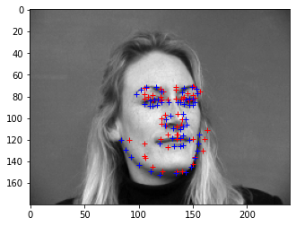 Good example #1
|
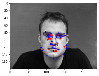 Good example #2
|
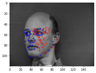 Bad example #1
|
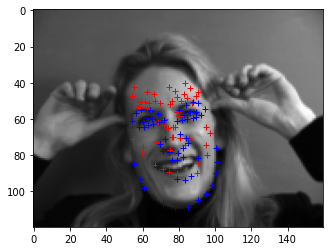 Bad example #2
|
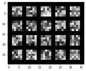
Below are the filters learned for the first convolutional layer:
Part 3: Train with Larger Dataset
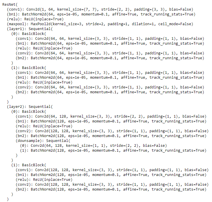
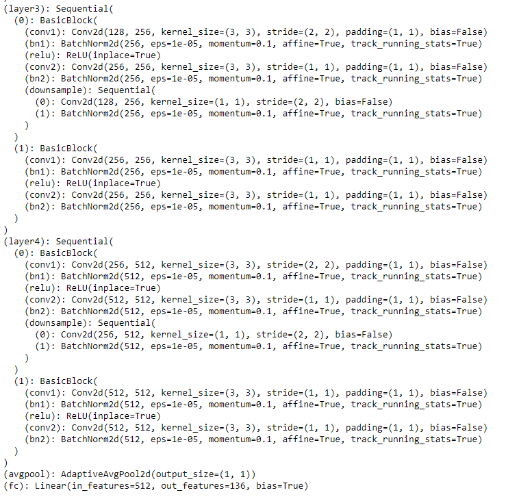
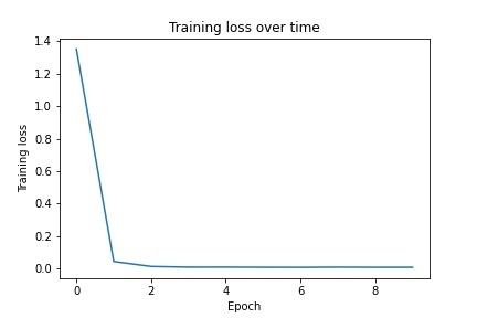
For part 3, I chose to use ResNet for training on the dataset. I modified my dataloader to output the portion of the image within the bounding box as the samples with the points normalized within the bounding box to train on. I modified ResNet to accept 1 layer (greyscale) and output 136 values (68x2). I used a learning rate of 0.01 and ran for 10 epochs. Below is the architecture of the net as well as graphs of the training/validation loss:
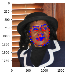
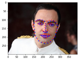
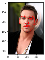
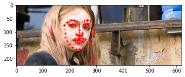
I then ran my model and submitting to Kaggle, and received a mean absolute error of 25.25994. Below are five images results from runnning the net, three of which are from the validation set and two of which are from the Kaggle submission set. One of the images from the validation set has a poor result, which I believe may be because of the leftwards orientation of the face. In the below images, the blue point is the ground truth and the red point is the predicted value:
 Validation example #1
|
 Validation example #2
|
 Validation example #3 (bad)
|
 Training example #1
|
 Training example #2
|
Bells & Whistles: Fully Convolutional Neural Net
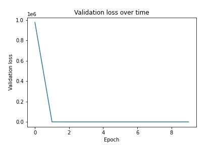
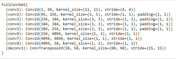
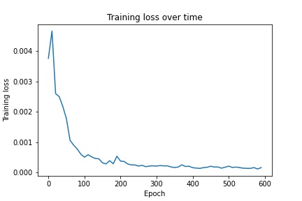
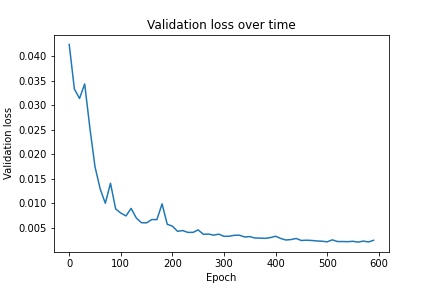
For the bells and whistles portion of the project, I implemented a fully convolutional neural net that I based off of AlexNet. I chose AlexNet because it is a relatively simple model that I could extend into a fully convolutional version. To do this I replaced all fully connected layers with convolutional ones that used 1x1 filters. Because the result is much smaller than the original image size, I use a transpose convolution operation to upscale the output back to 240x180. Following this, the output of the net is a single image sized heatmap for each keypoint that predicts the probability of a keypoint existing in each pixel. To make a prediction on a keypoint, I took the argmax of its corresponding heatmap. In order to train the model on an image, I generated a 2d heatmap for each ground truth keypoint, with a gaussian kernel centered at the location of the keypoint. I used a learning rate of 0.001. Below is the architecture of the model as well as the training/validation losses:
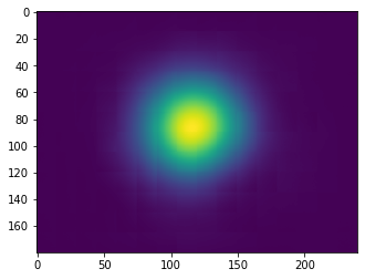
Below are two examples of ground truth point heatmaps against the heatmaps generated by the net:
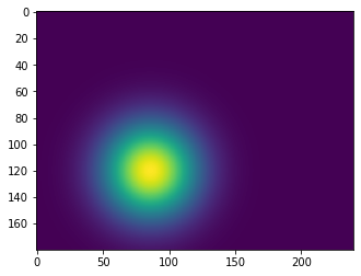 Ground truth for point #1
|
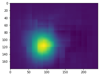 Heatmap output for point #1
|
 Ground truth for point #2
|
 Heatmap output for point #2
|
Below are two examples of image outputs generated by the fully convolutional neural net. In the below images, the blue point is the ground truth and the red point is the predicted value: