|
In this project, I implemented "A Neural Algorithm of Artistic Style" (Gatys et al.). The paper uses neural representations to separate and recombine content and style of arbitrary images, thus creating images in the style of another. Specifically, the layers in a Convolutional Neural Network (CNN) can be understood as a collection of image filters, each of which extracts a certain feature from the input image. The paper highlights the higher layers that learn the content (objects and their arrangement rather than pixel values) of an image, and a feature space consisting of the correlations between the different filter responses over the spatial extent of the feature maps that captures texture information rather than global arrangement. By tuning weights that trade-off between specific loss functions (below) of the content and style, one creates new stylized images.
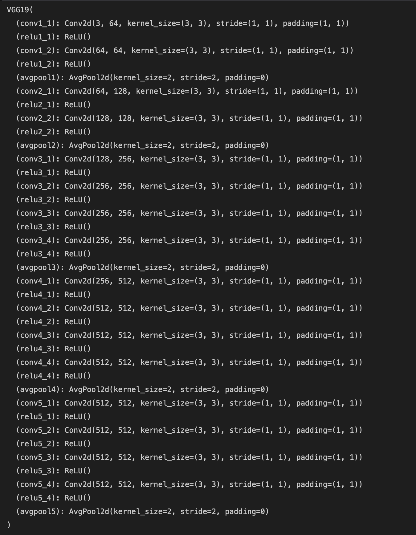
As the paper suggests, I use a pretrained 19 layer VGG network with the max pooling layers replaced by average pooling layers and with the fully connected layers thrown out. The network is then modified so that it returns the layer activations after the specified layers in the paper (conv4_2, conv1_1, conv2_1, conv3_1, conv4_1, conv5_1).
|
|
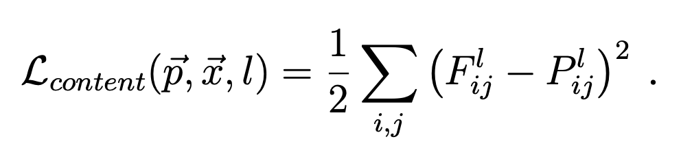
A given input image is encoded in each layer of the CNN by the filter responses to that image. The paper defines the content loss between the content image and the generated image at a certain layer as the squared-error loss between the two feature representations at that layer:
|
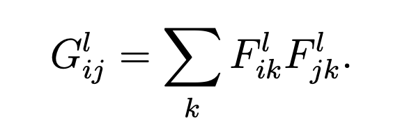
where p and x are the original image and the image that is generated and P^l and F^l their respective feature representation in layer l (the ith jth entry is the activation of the ith filter at index j). In order to obtain a style representation, at each layer we compute the Gram matrix of the feature maps. In equations, the ith jth entry of the layer l matrix is given by the inner product of the vectorized feature map i and j at layer l:
|
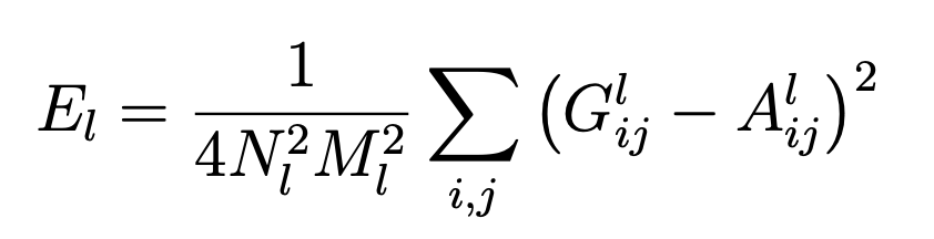
This Gram matrix measures the correlations between the different filter responses regardless of their location in the image, which is precisely what encodes style. The style loss is then defined to be the weighted sum of the normalized mean squared errors between the gram matrices of the style image and the generated image at various layers. In equations:
|
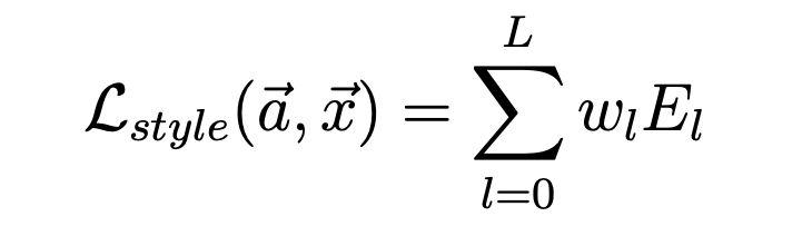
|
where a and x are the original image and the generated image and A^l and G^l their respective style representations in layer l, w_l are the weighting factors of the contribution of each layer to the style loss, N_l is the number of filters at layer l, and M_l is the size of each filter at layer l. The total loss is then the weighted sum of the content and style losses (weights alpha and beta are tuned to have a resulting image with the desired amount of content and style: a lower ratio gives more weight to the style image and a higher ratio gives more weight to the content image). The equation is given by the following:
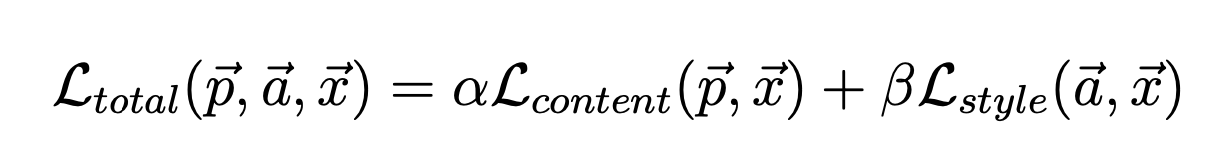
|
where p, a, and x are the content image, style image, and generated image respectively.
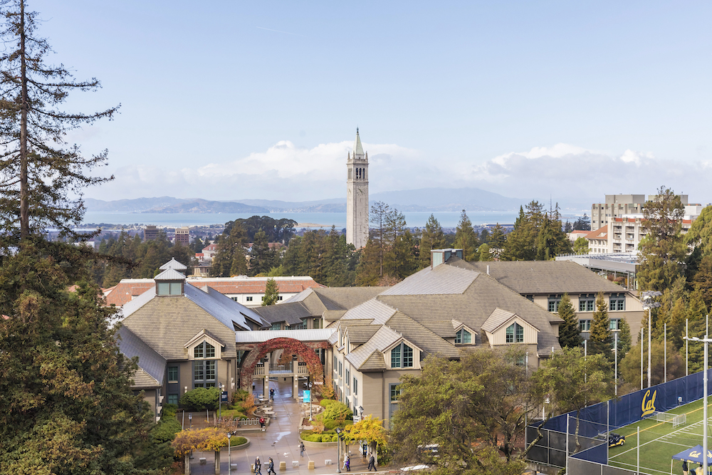
To generate images that mix the content of one image with the style of another, the paper suggests jointly minimizing the distance of a white noise image from the content representation of the content image in one layer of the network (conv4_2) and the style representation of the style image in a number of layers of the CNN (conv1_1, conv2_1, conv3_1, conv4_1, conv5_1) (i.e. minimize the total loss function above with gradient descent). I found that starting with the content image instead of a white noise image gave less noisy and nicer looking results. I also found that significant tuning of the alpha-beta ratio was necessary to produce good-looking results. Below, I use the LBFGS optimizer with default parameters for 15 epochs and alpha-beta ratios as indicated.
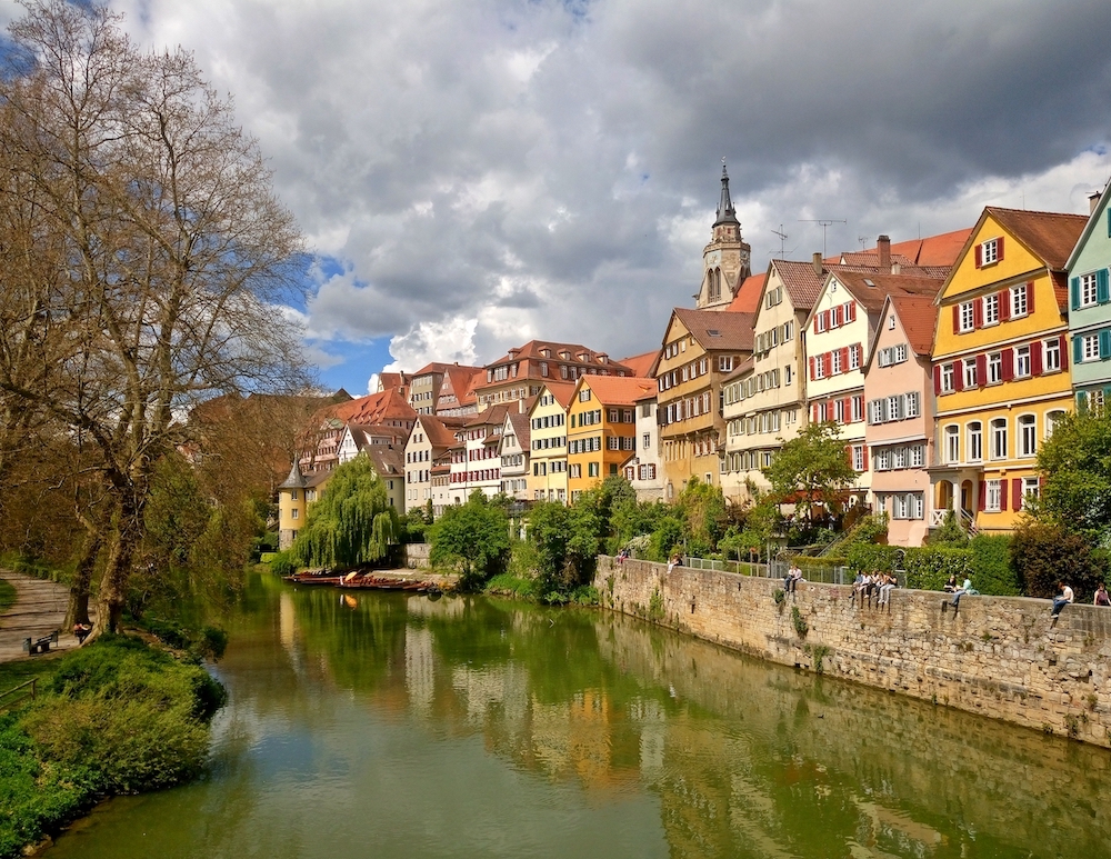
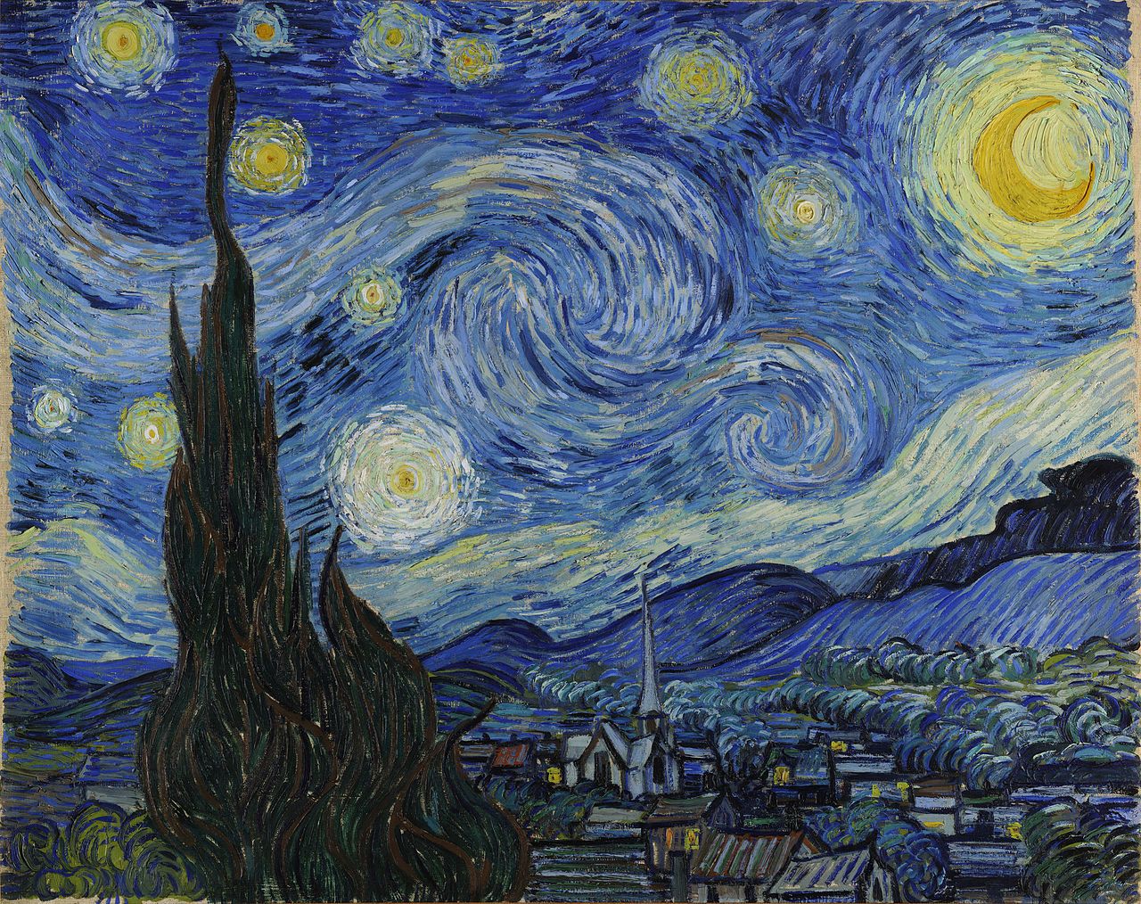
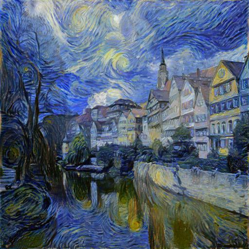
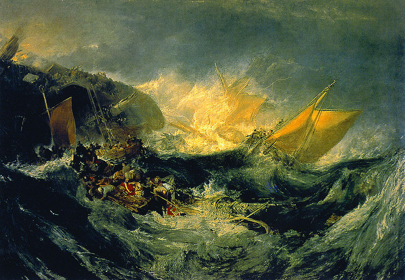
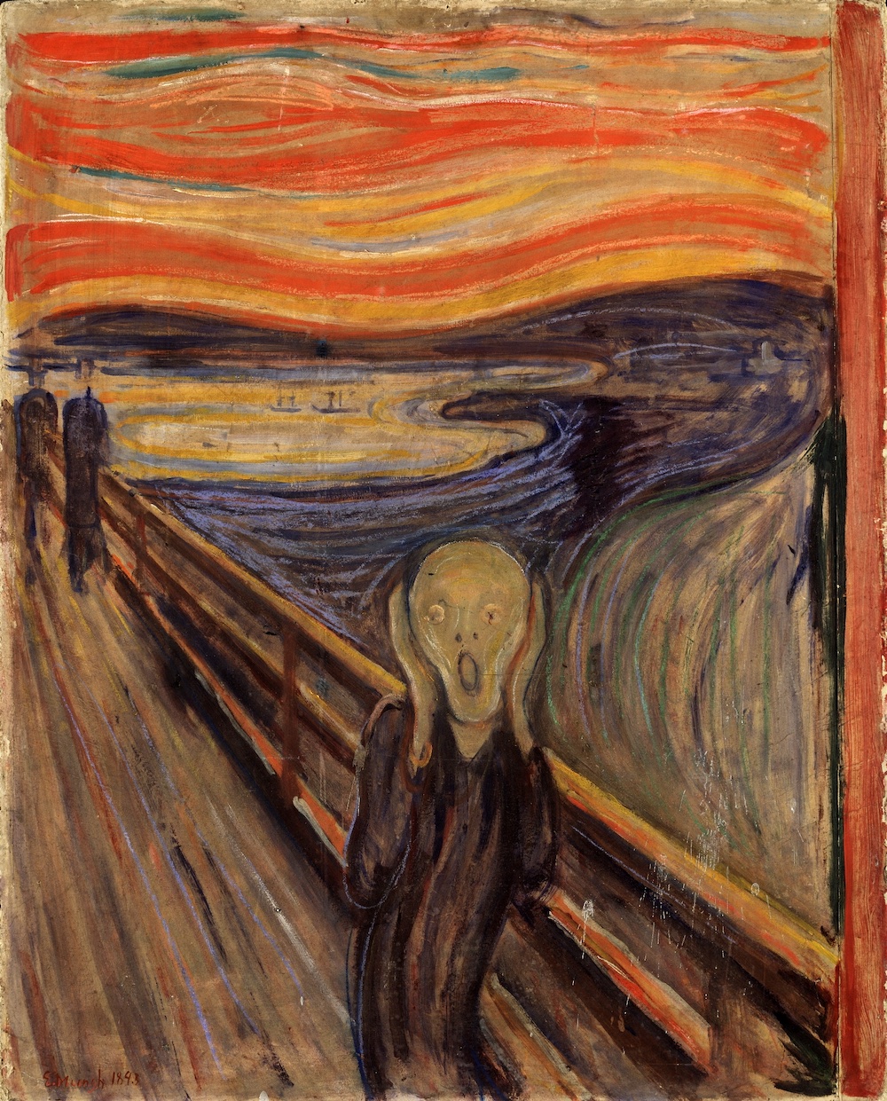
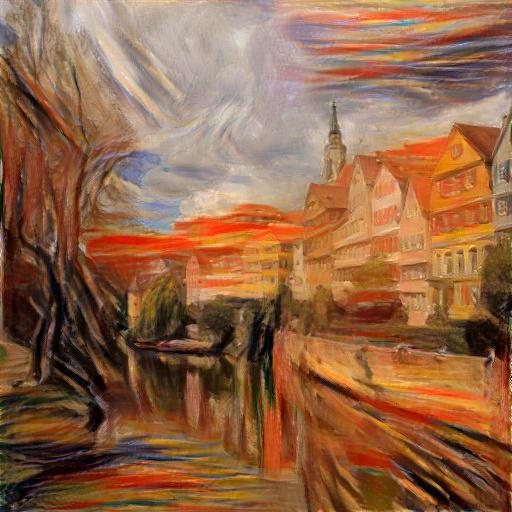
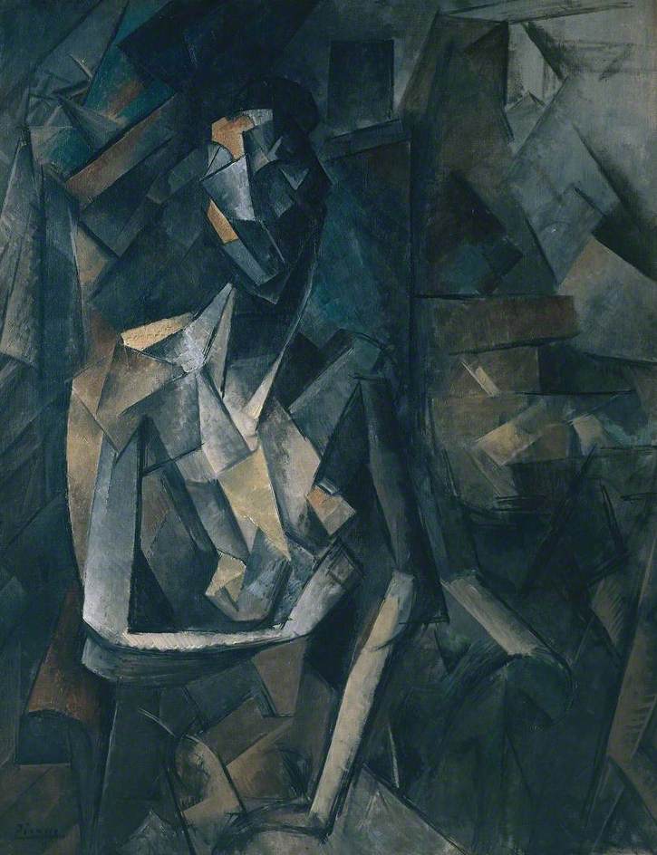
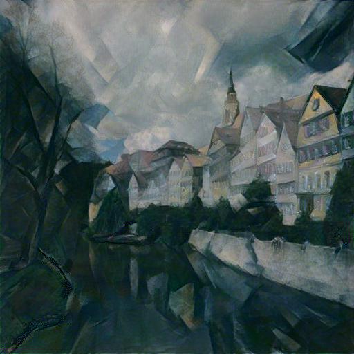
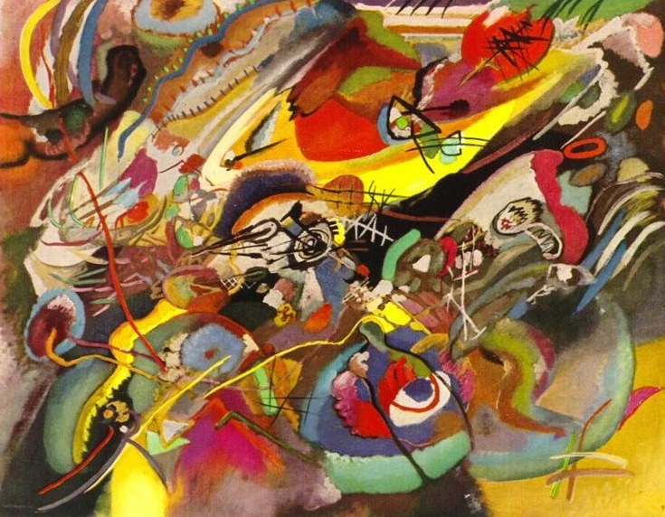
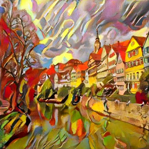
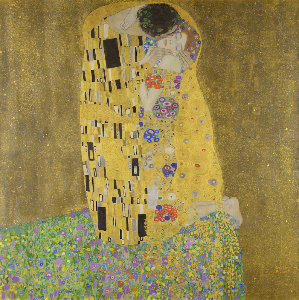
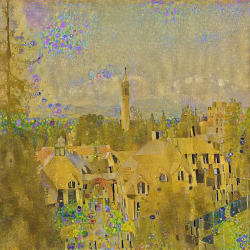
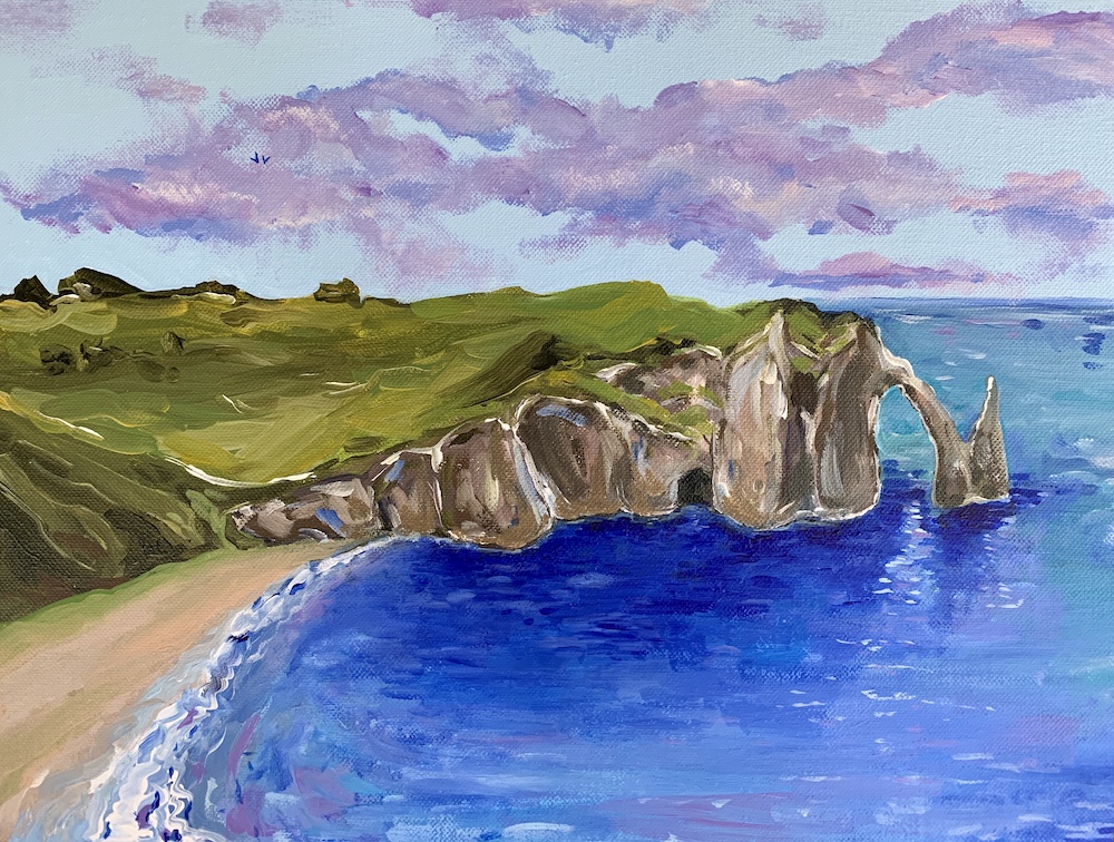
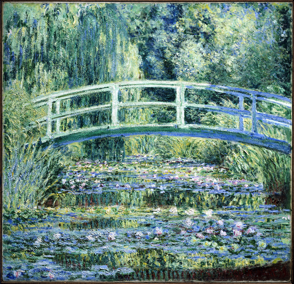
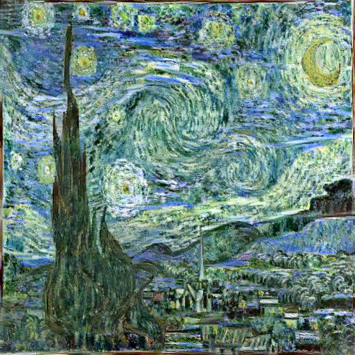
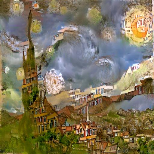
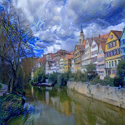
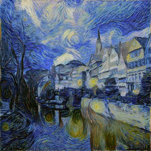
The following are recreations of figure 2 in the paper:
|
|
|
|
|

|
|
|
|
|
|
|
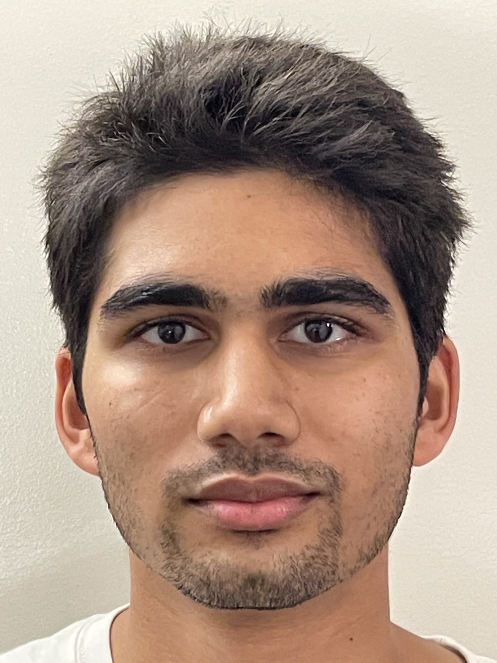
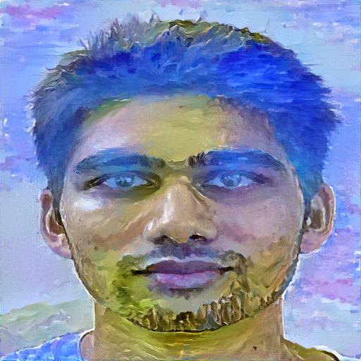
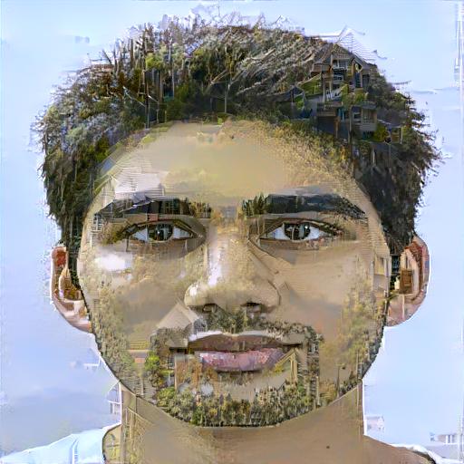
The following are my own creations using the project.
|
|
|
|
|
|
|
|
|
|
Some notable failure cases include using artwork as the content image and a photograph as the style image, and using photographs as both the content and style images. This is likely due to the fact that if the style image is a photograph, then there aren't enough repeated patterns in the image to derive a style that can be transferred. Also notable are the dramatic changes that differences in the alpha-beta ratio make. Finally (not shown), it was interesting to see how the algorithm affected images of different sizes differently. When using smaller images, a larger ratio was necessary, but with larger images a smaller ration was needed (and the images looked better stylized).
|
|
|
|
|
|
|
|
|
|
|
|
|
|
|
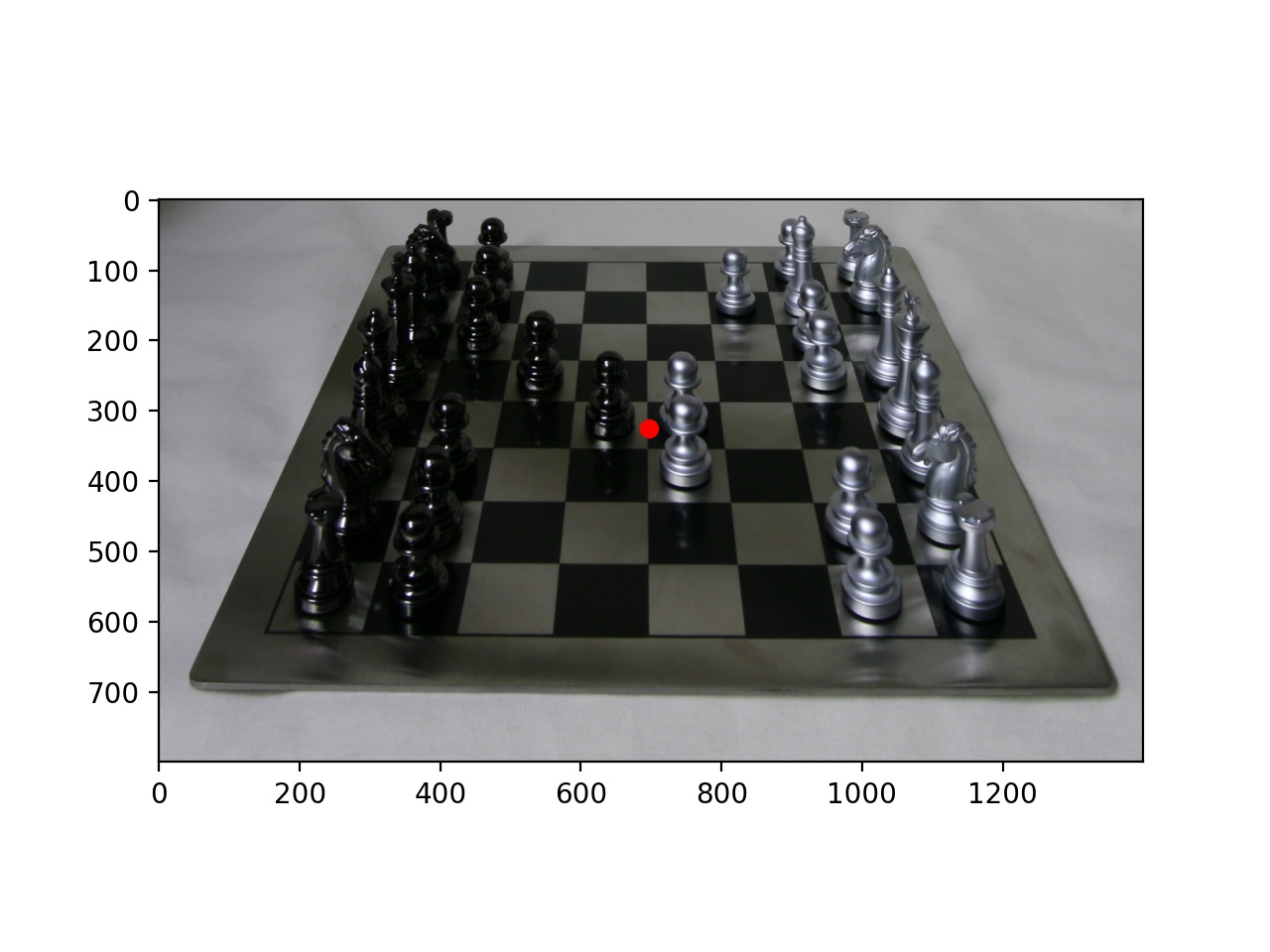
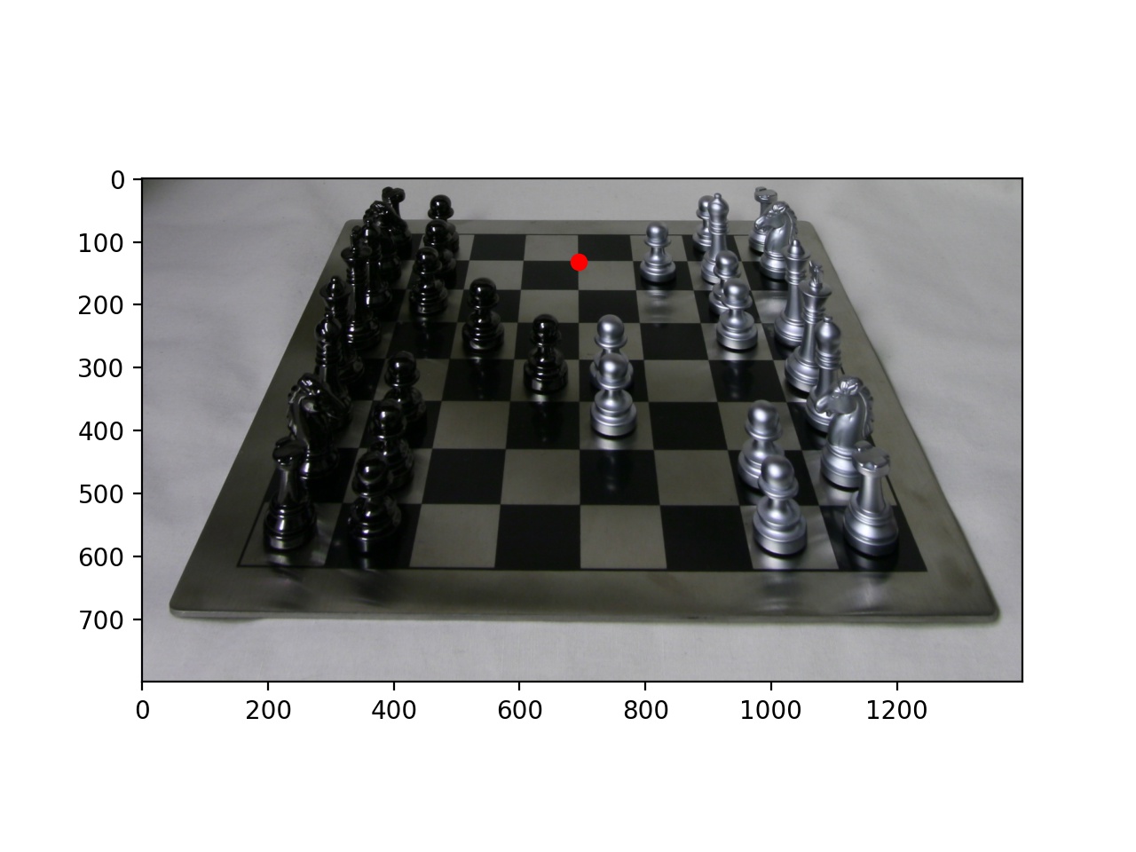
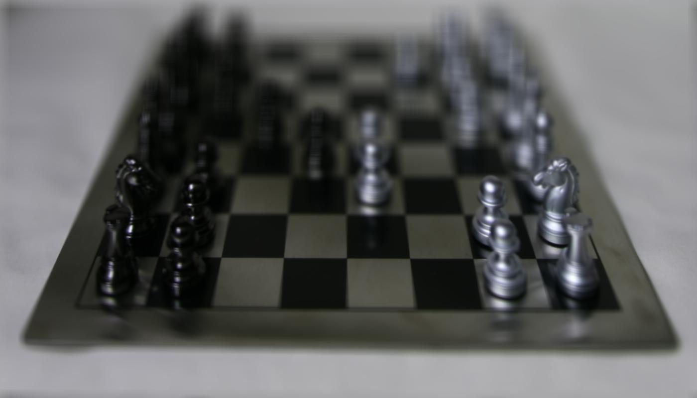
In this project, I used lightfield data (multiple images captured over a plane orthogonal to the optical axis) and create complex effects (in this case depth refocusing and aperture adjustmnt) using simple operations like shifting and averaging. I used the chess lightfield data from the Stanford Light Field Archive (289 views over a 17x17 grid) as my dataset.
From these images, we have a fixed position of the image plane while varying the position of a camera over a grid. Each camera captures light at a slightly different angle. The objects that move the least between camera shots are thus those at the furthest depth. So, to achieve a focusing effect, the image set of light rays are aligned and integrated over a single pixel, for every pixel in the image. The alignment is done by shifting the images according to the difference between the camera coordinates in the filenames and some reference image. In this case, I use the center image (at position (8, 8) in the light field). To achieve varying depths, I apply a constant multiplier to the x and y shifts for every image. The lower the multiplier, the farther back the focus is, and the higher the multiplier, the closer the focus is. The gif below was generated by varying this multiplier over the range [-.1, .7].
|
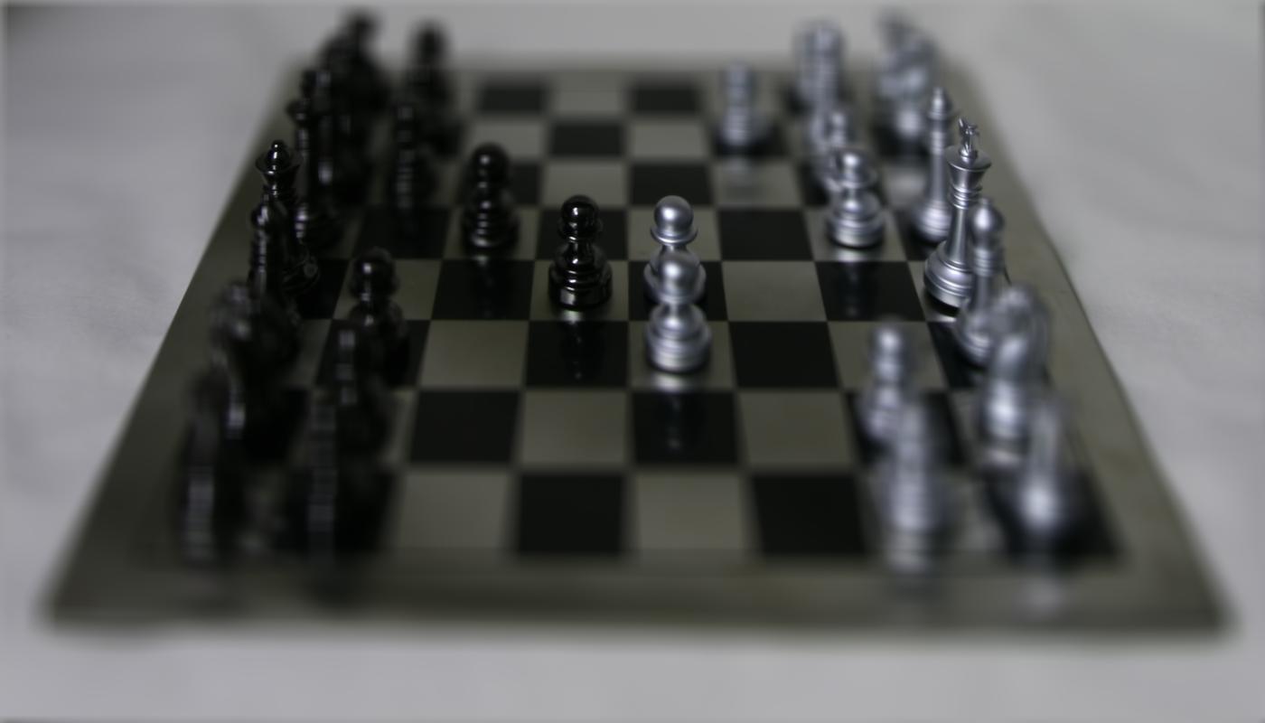
For this part, I fix the focus depth at .3 (middle of the image) to highlight the effect of changing the aperture. The images are aligned just as in depth refocusing. Since each image contains the light captured, in order to increase aperture, I average more images. The smallest aperture is thus given by a single image. To simulate a larger aperture, need more light rays to average, so I take a box of a certain radius around the single image and average them. I choose the center image as the smallest aperture image as it gives the smoothest transition and the most radii to work with. The gif below was generated by varying this radius over the range [0, 7].
|
For the Bells and Whistles on the Lightfield project, I chose to implement interactive refocusing. The focusing depth depends on the multiplier on the shifts. Following the depth range found above, I linearly interpolate the y coordinate to the depth range and apply the refocusing algorithm at that depth.

|
|
|
|
|

|
I was amazed at how simple shifting and averaging operations were able to make complex operations like refocusing and aperture adjustment after the images are taken. It was impressive to see that a lightfield, which is simply images of the same scene taken from slightly different positions, enables advanced post-processing effects.