Gradient Domain Fusion

Introduction

When blending two images together, the simplest technique would be to directly copy and paste the pixel values from one image to the other. However, incompatibility between the source and the target would result in noticable seams in the resulting image.

One way to remedy this issue is to use gradient domain fusion (Poisson blending). This technique utilizes the fact that when looking at an image, we pay more attention to the rate of change (gradient) instead of the exact pixel values. Forcing the gradient of the resulting image to match the source and target image respectively would allow a smooth transition from one theme to the other.

Toy Example: Recovering the Image

As a warm-up, we will first try recovering the original image using least squares, constraining on $x$$x$-gradients, $y$$y$-gradients and pixel values. In particular, we want the $x$$x$-gradient differences, $y$$y$-gradient differences and color distortion between the original and generated image to be as small as possible. Sucn goal can be written as three objectives:

During implementation, we can first construct a sparse matrix that calculates the $x$$x$-gradient for every pixel in the image, and another sparse matrix that calculates their $y$$y$-gradient. A matrix $A$$A$ can be constructed by concatenating the two gradient matrices together, along with $\left[\begin{array}{c}1\overrightarrow{0}\end{array}\right]$$\begin{bmatrix} 1 \quad \vec{0}\end{bmatrix}$ to make sure that the colors align. The least squares problem can be written as: $A\overrightarrow{v}=\overrightarrow{b}$$A \vec{v} = \vec{b}$, where $\overrightarrow{b}$$\vec{b}$ contains the $x$$x$-gradient, $y$$y$-gradient and upper-left pixel value of the source image. The resulting image can be recovered by reshaping the 1D vector $\overrightarrow{v}$$\vec{v}$ into a 2D image.

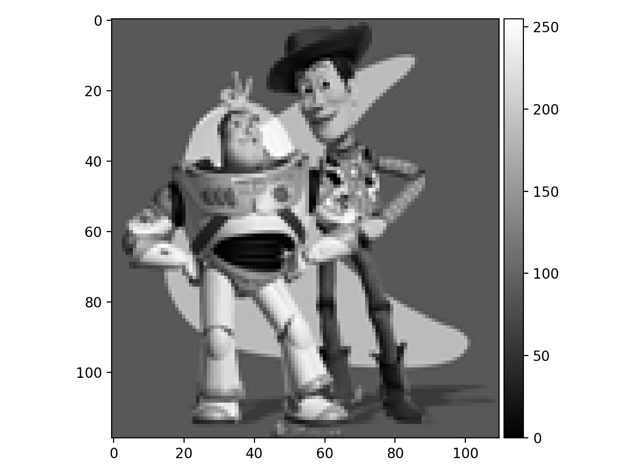
To test the correctness of our implementation, the original image is presented below:

The resulting (recovered) image is as follows:

Poisson Blending

In this part, we are going to use gradient information to seamlessly blend two images.

The first step is to select the source and target regions. We need to first specify a patch in the source image that we would like to blend, as well as its desired location in the target. The source image should then be transformed to match its selected region with the target location. We will impose a mask on both source and target image to extract the desired region and place it in the correct location.

Poisson blending can be performed after alignment. We'll try to ensure that the gradient of the resulting image match closely with the source image for pixels in the mask, and aligns with the target image for pixels outside the mask. This means that for pixels outside the masked area can be directly copied from the target image. Pixel values inside the masked area should be calculated by gradient matching. We will calculate left, right, up and down gradients for each pixel. Calculation of gradiet is divided into two situations: if the neighboring pixel is within the masked area, the gradient would be value of the current pixel minus the value of the neighboring pixel. Otherwise, the gradient would be value of the current pixel minus the value of the corresponding target pixel.

The final objective would be like this:

During implementation, we can regard $\overrightarrow{v}$$\vec{v}$ as a flattened image. We will set up a sparse matrix as in the previous part that calculates the left, right, up and bottom gradients. We will also have a vector $\mathrm{\Delta }s$$\Delta s$ that records the gradients in the source image, as well as an offset vector $\overrightarrow{o}$$\vec{o}$ that records whether we will use pixel values in the target image. i.e., $o_j$$o_j$ will be $t_j$$t_j$ if we the current pixel is at the boundary, and its neighboring pixel location $j$$j$ is outside the masked area; $o_j$$o_j$ will be $0$$0$ otherwise.

The least squares problem can be written as: $A\overrightarrow{v}-\overrightarrow{o}=\overrightarrow{b}$$A \vec{v} - \vec{o} = \vec{b}$, where $\overrightarrow{b}$$\vec{b}$ is the left, right, up and down gradients for each pixel in the masked region of source image. Solving for the least squares problem can give us pixel values within the masked region of the resulting image. We can then iterate through all pixel locations and fill in the masked region.

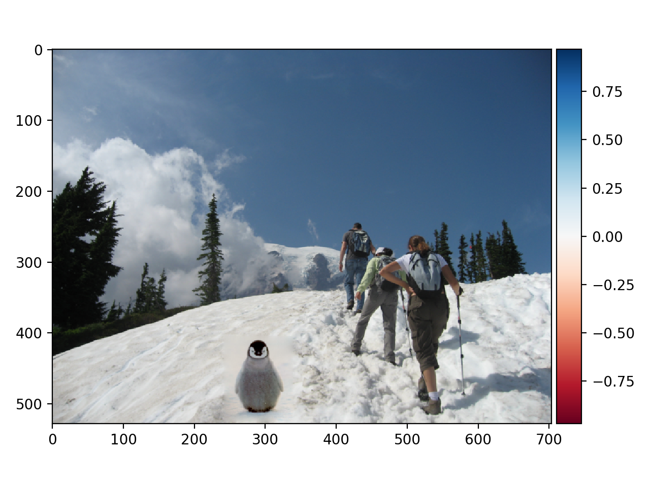
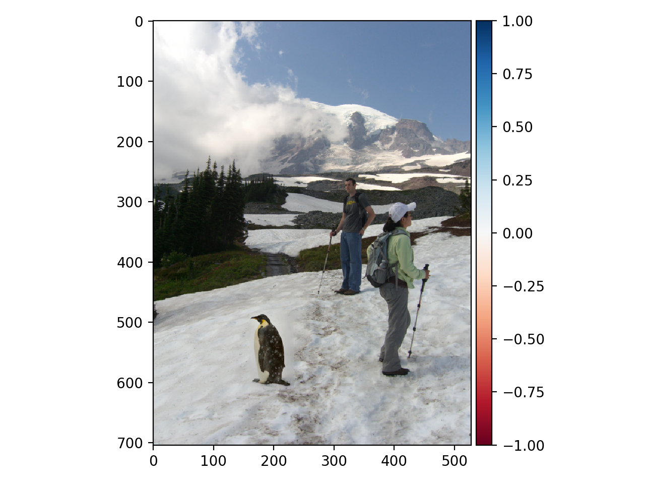
Here are three groups of source and target images as well as the blended resulting image:

Penguin chick and Hikers:

Penguin and Hikers:

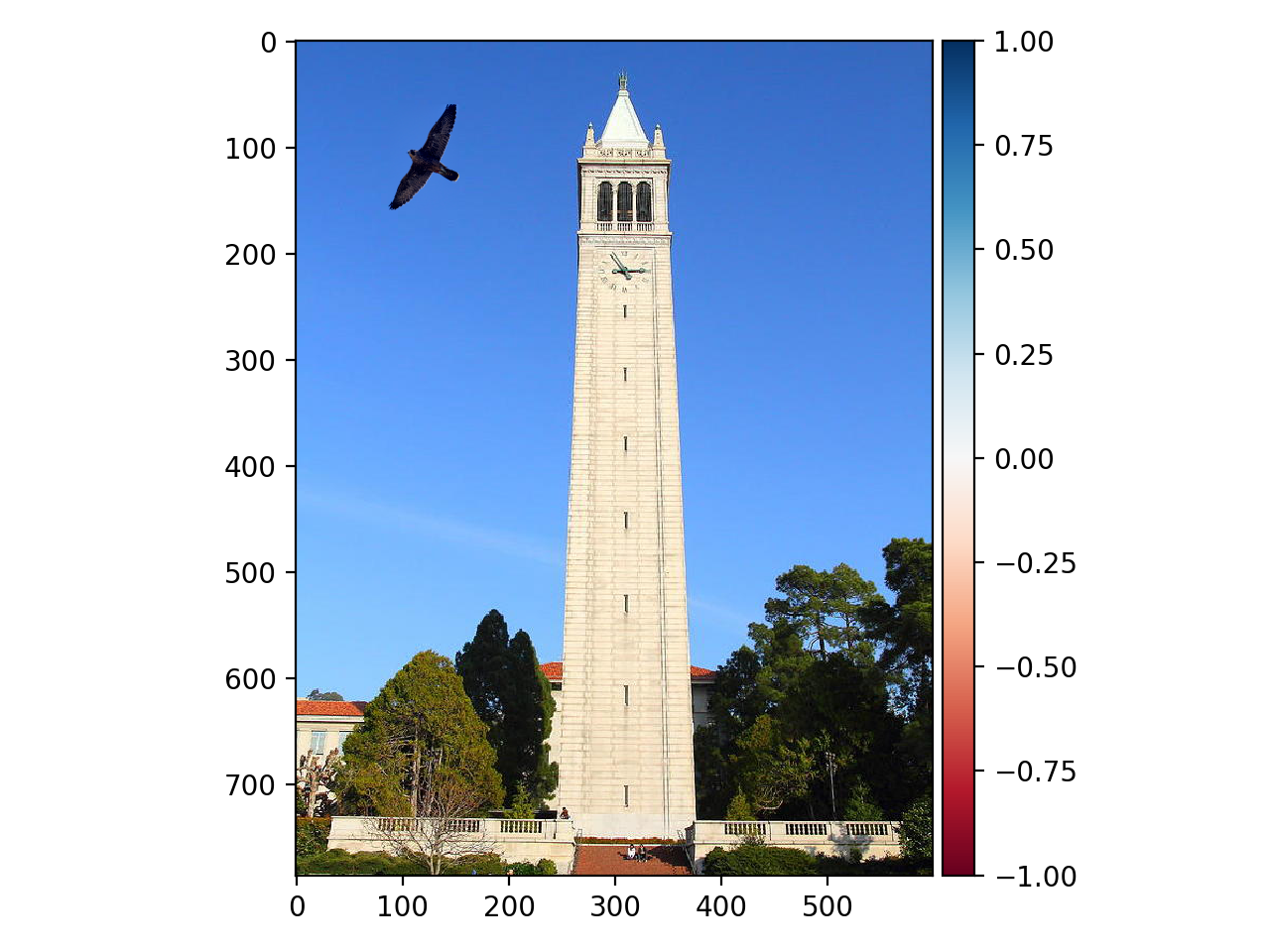
Falcon and the Campanile:

Mixed Gradients

In this part we will investigate an updated technique of Poisson blending. Instead of forcing the gradients of resulting image to align with those of the source image, we will now pick the larger gradient value between the source and target image. In other words, the objective function becomes:

where $d_{ij}=s_i-s_j$$d_{ij} = s_i - s_j$ if $|s_i-s_j|>|t_i-t_j|$$\abs{s_i - s_j} > \abs{t_i - t_j}$, and $d_{ij}=s_i-s_j$$d_{ij} = s_i - s_j$ otherwise.

During implementation, we will keep the gradient matrix $A$$A$ and offset vector $\overrightarrow{o}$$\vec{o}$ the same as regular Poisson blending, and let $\overrightarrow{b}$$\vec{b}$ be the elementwise larger value between the gradient of $\mathbf{s}$$\mathbf{s}$ and gradient of $\mathbf{t}$$\mathbf{t}$.

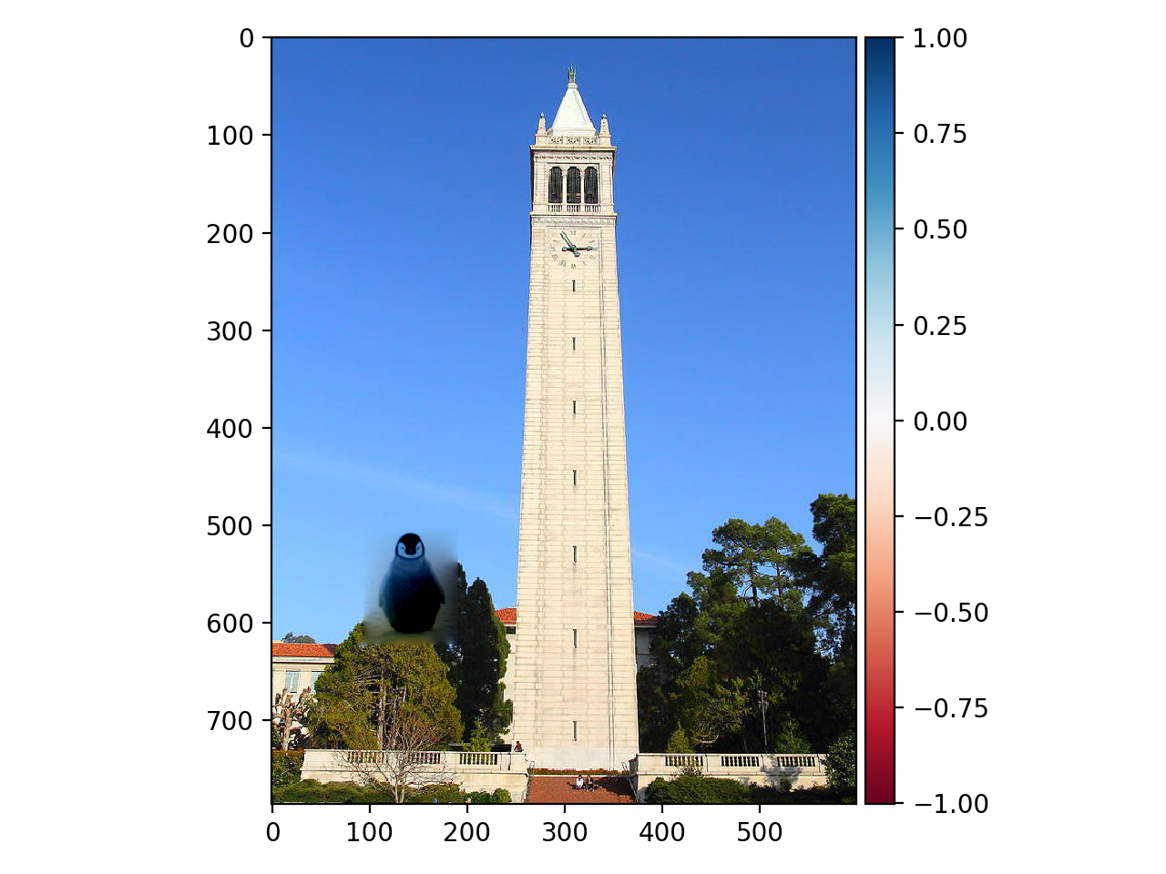
To visualize the differences between mixed gradients and regular Poisson blending, we can investigate the results for blending two images with significantly different background colors using these two methods respectively. Here we will produce a "crazy" image of blending the penguin chick onto a tree beside Campanile.

Regular Poisson blending:

Mixed gradients, Penguin on the tree:

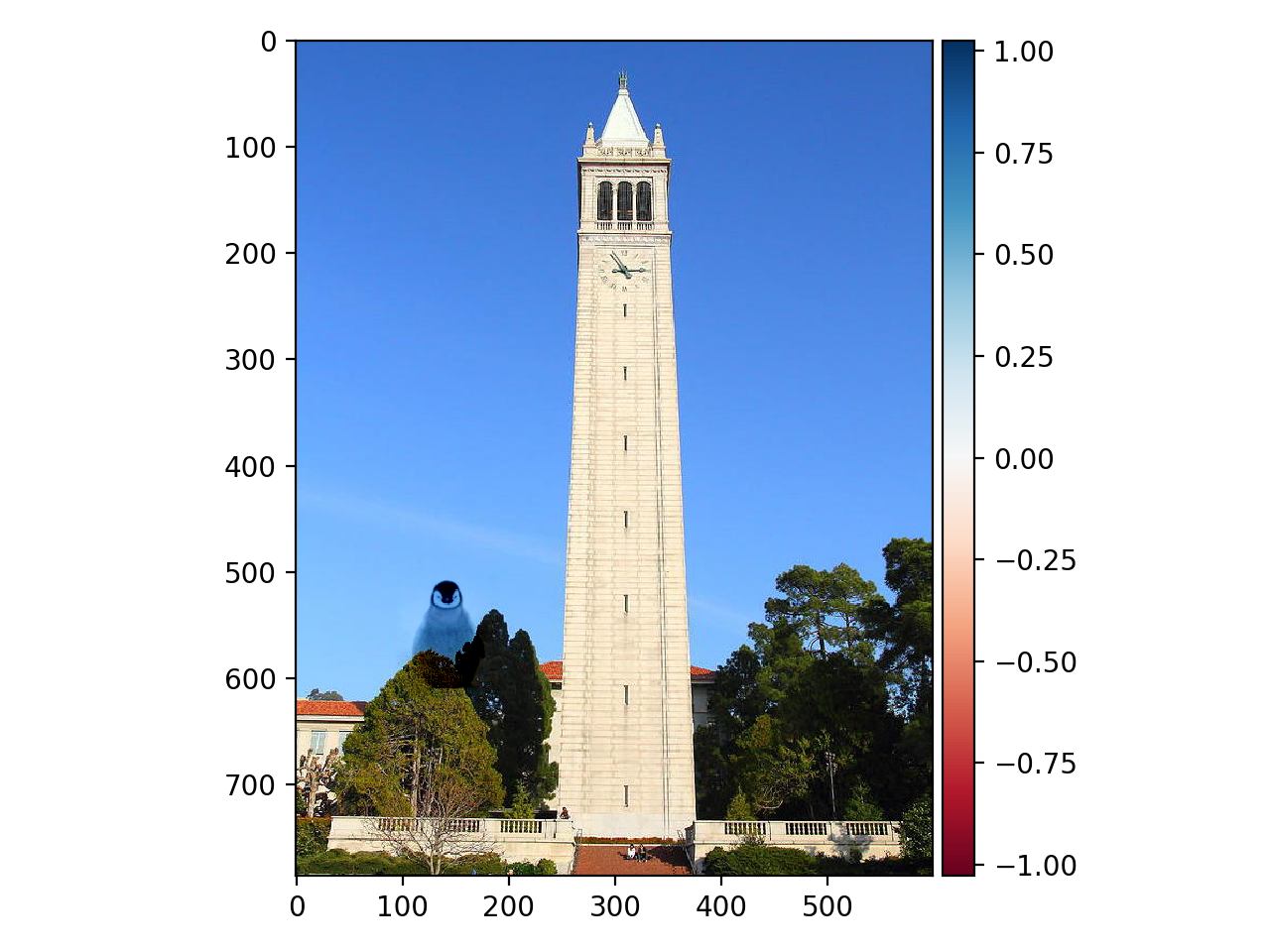
We can see that mixed gradient method produces smoother transition from background to source image. This is because mixed gradient method always follows the most significant change in pixel value. When background has sharper contrast than the source image, it will manage to align source image pixel values with the background and produce better blending results.