Final Project 1: Image Quilting
Comparison of Quilting Techniques
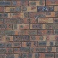
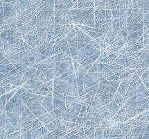
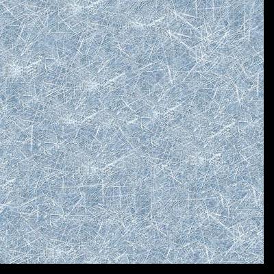
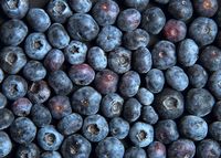
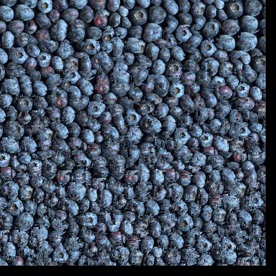
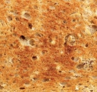
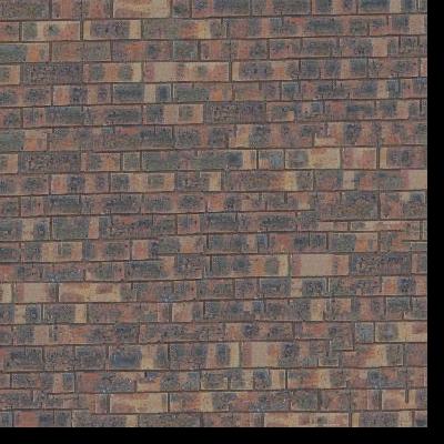
Original
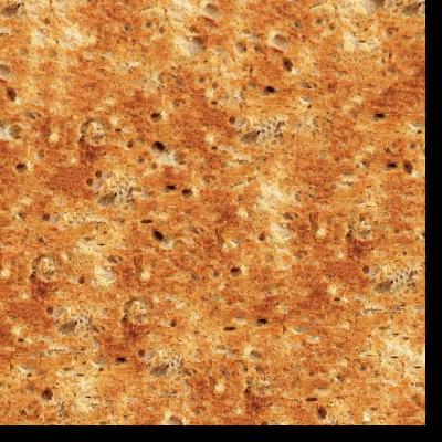
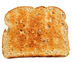
Random Quilt
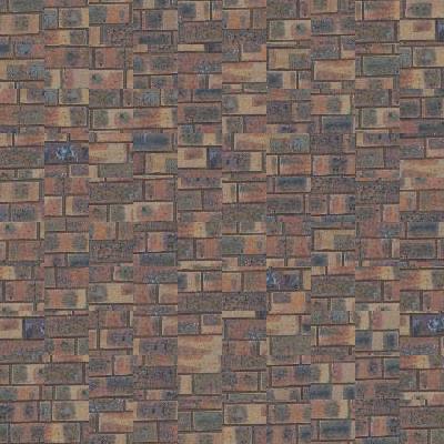
Overlapping Quilt
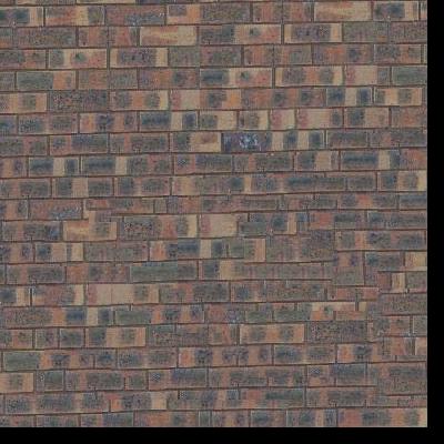
Seam-Finding Quilt
Seam Finding
Below are two patches that overlap for the brick wall. The cost image has the min-cost path shown in white.
For this particular overlap, it happens to be so similar that the errors are very low and occur at the leftmost edge.

Overlap Region 1

Overlap Region 2

Cost image with min-cost path
The image quilting technique consists of first finding the patch that is most similar in the overlap region. Then
instead of directly copying that patch onto the quilt, we find the min-cost path which provides the ragged boundary
between the two overlapping patches that best stiches the two patches together. This min-cost path is found through
dynamic programming, considering the cummulative error along all possible paths. In the case of vertical boundaries
as shown in the example above, pixels left of the min-cost path are pixels from overlap region 1 and those right of
the min-cost path are pixels from overlap region 2. This process is repeated until the entire quilt has been filled
with patches.
A difficulty I encountered was writing the min-cost path algorithm on my own for the Bells & Whistles. It was also
more difficult to get a synthesized texture that looked more natural for textures that were bigger, like the berries.
A design decision I made was to make the patch sizes 25 by 25 with an overlap region of 5 pixels.
Seam Finding Results
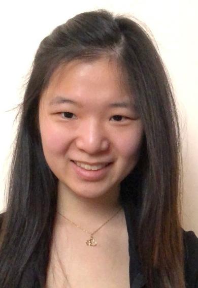
Texture Transfer
To transfer the texture from a source image onto a target image, first construct correspondence maps.
I used the luminosities as the correspondences. For each patch of the target image, look at the corresponding
patch in the luminance correspondence map C1. Then find the best match for C1 in the luminance correspondence
map for the source texture image, and say the best matching patch is C2. The patch corresponding to C2 in the
source image is stiched into the target image using the seam-finding quilting technique illustrated above.
A difficulty I encountered was deciding on the correspondence map, but I ultimately settled on what the paper
used which was just the luminance of the pixels. As a design decision, I chose to stick with the sketch texture,
because there are enough differences in the texture to paint more details. However, without the iterative method
described in the paper, the end result does not look as seamless.
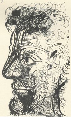
Texture
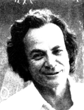
Target Image
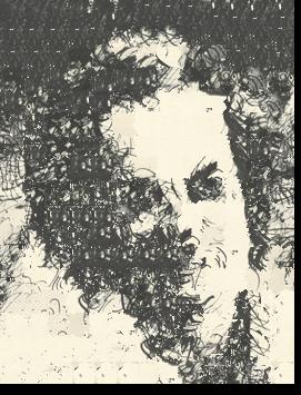
Result
Texture
Target Image
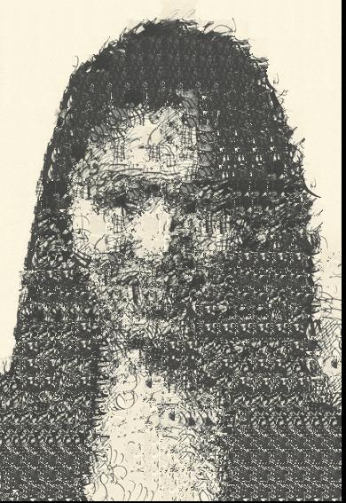
Result
Bells & Whistles
Create and use your own version of cut.m.
I created my own version of cut.m using dynamic programming in python. The code can be found in the function
_min_error_cut of the main.py file in image_quilting. I implemented two versions depending on whether the seam
was vertical or horizontal.
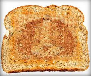
Face on toast
I used texture transfer to recreate the dog face with the toast texture. Then I used Laplacian pyramid blending
to put that dog face onto toast.
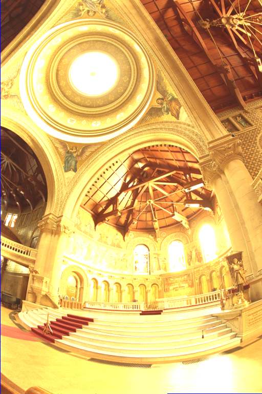
Final Project 2: High Dynamic Range Images
Original Images
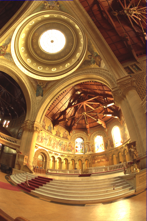
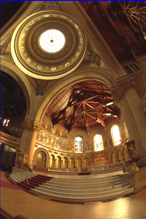
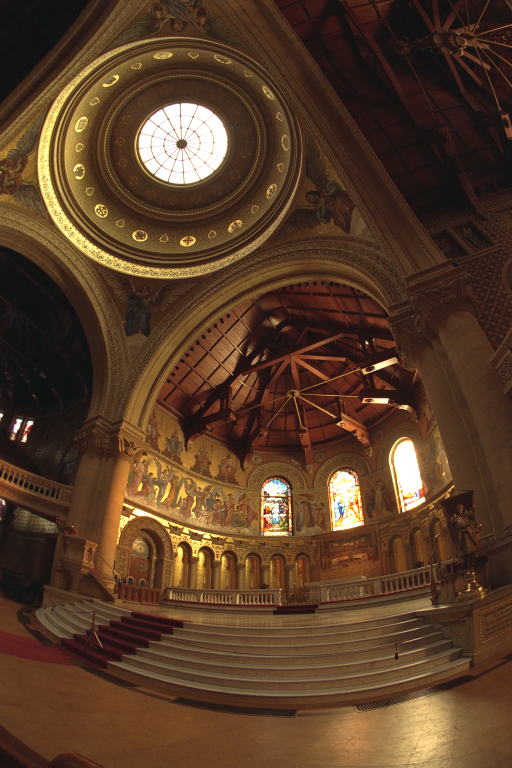
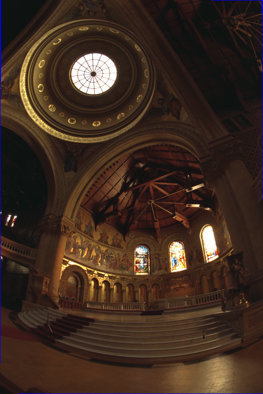
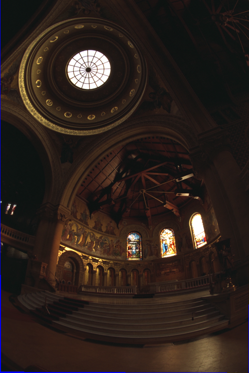
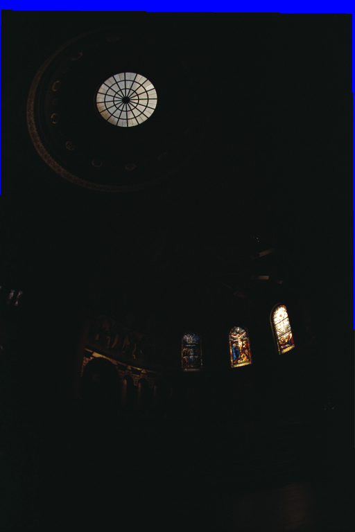
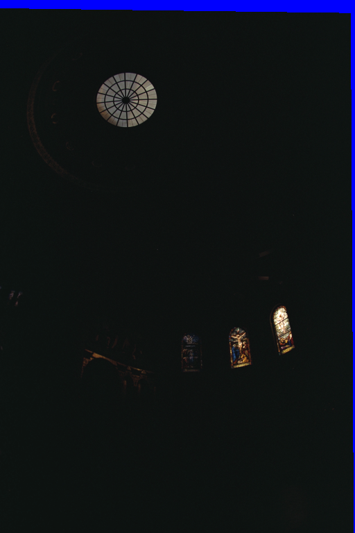
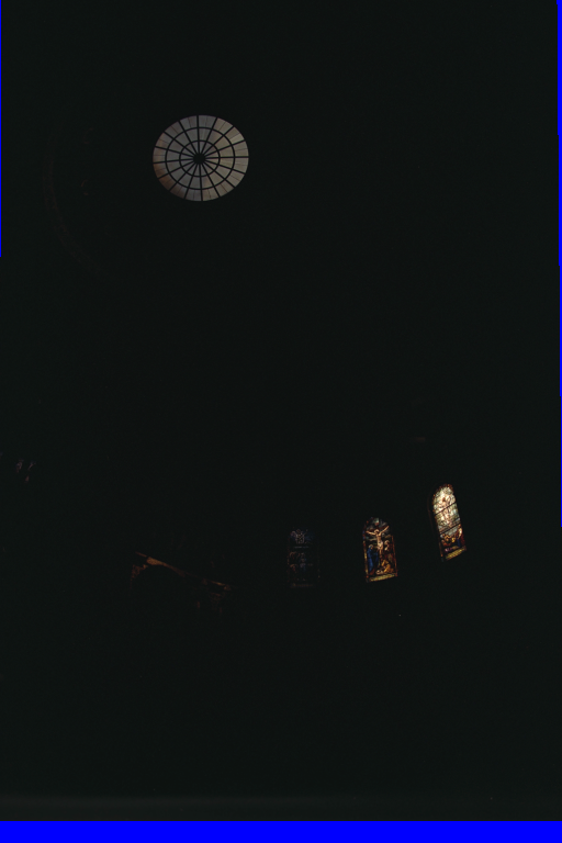
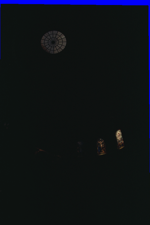
Below are the original images with different exposure times that are used to construct the HDR image.
Exposure: 32.0
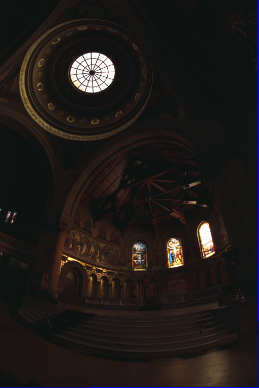
Exposure: 16.0
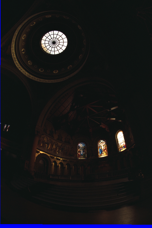
Exposure: 8.0
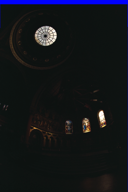
Exposure: 4.0
Exposure: 2.0
Exposure: 1.0
Exposure: 0.5
Exposure: 0.25
Exposure: 0.125
Exposure: 0.0625
Exposure: 0.03125
Exposure: 0.015625
Exposure: 0.0078125
Exposure: 0.00390625
Exposure: 0.001953125
Exposure: 0.0009765625
Radiance Map Construction
Following the algorithm described in the paper by Debevec and Malik 1997, I solved for the log of irradiance
values ln E_i and the function g in the system of equations
g(Z_ij) = ln(Ei) + ln(delta_t_j)
where Z_ij is the
ith pixel from picture j, and delta_t_j is the exposure time for picture j. I sampled over 50 pixels from each
of the images to construct the matrix Z. I also followed the paper to add weightings to emphasize the smoothness
of the curve and to fit terms towards the middle.
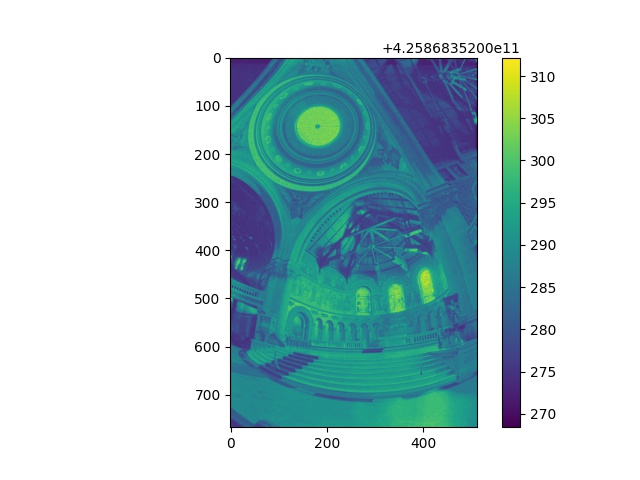
Below is the result of using the solved information to get the radiance for each pixel.
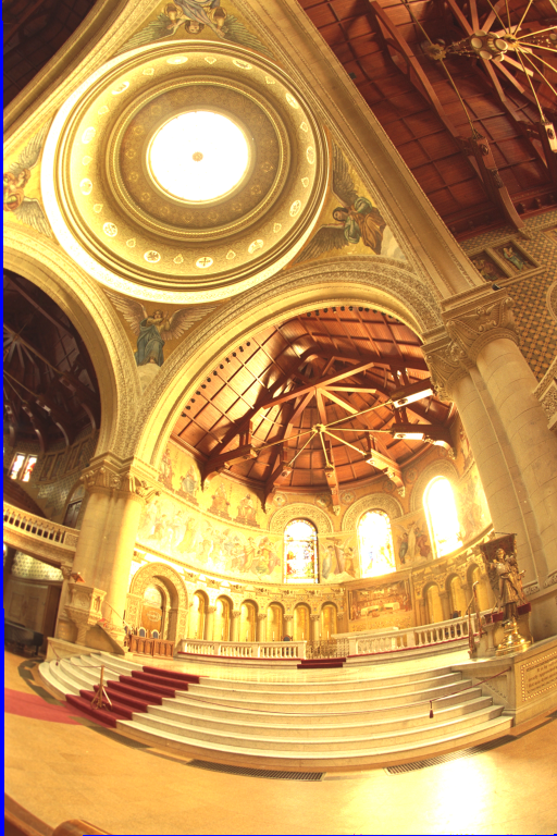
Tone Mapping
Following the simplified version of the algorithm in Durand 2002, I used the radiance map to get the intensity
of the pixels and the chrominance of each channel. Then I computed the log of the intensity and filtered it with
a bilateral filter, which smooths the noise while preserving the edge details. Then I separated the details layer
from the large scale structures (shown below), and applied an offset and scale to that base layer. Finally, I
reconstructed the log intensity and put back the colors with the chrominance channels and applied gamma compression
to the resulting image.
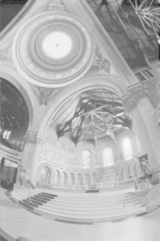
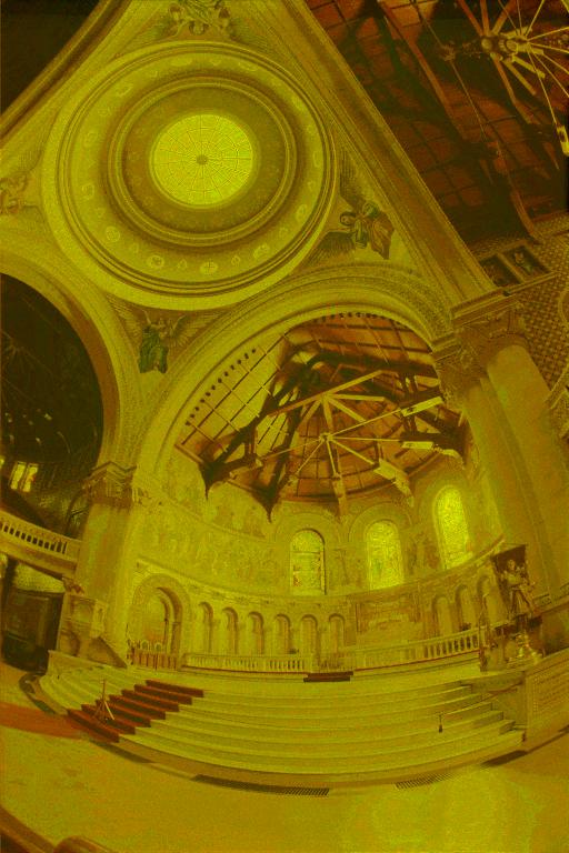
As shown below, the local tone mapping turned out better than the global tone mapping, which simply took a log of the
ln(E_i) of each channel and normalized.

Detail Layer
Base Layer (Large Structures)
Global Tone Mapping
Local Tone Mapping