Final Projects: Augmented Reality and Light Field Camera
COMPSCI 194-26: Computational Photography & Computer Vision
Professors Alyosha Efros & Angjoo Kanazawa
December 10, 2021
Ethan Buttimer
PROJECT 1: AUGMENTED REALITY
Summary
Augmented reality allows you to superimpose virtual objects onto real images or videos. The technique I used to achieve this relied on tracking algorithm to relate known 3D "world" coordinates to 2D image coordinates. With these correspondences, a camera projection matrix can be computed, then used to render the 3D objects we wish to place in the scene.
Setup and Keypoint Selection
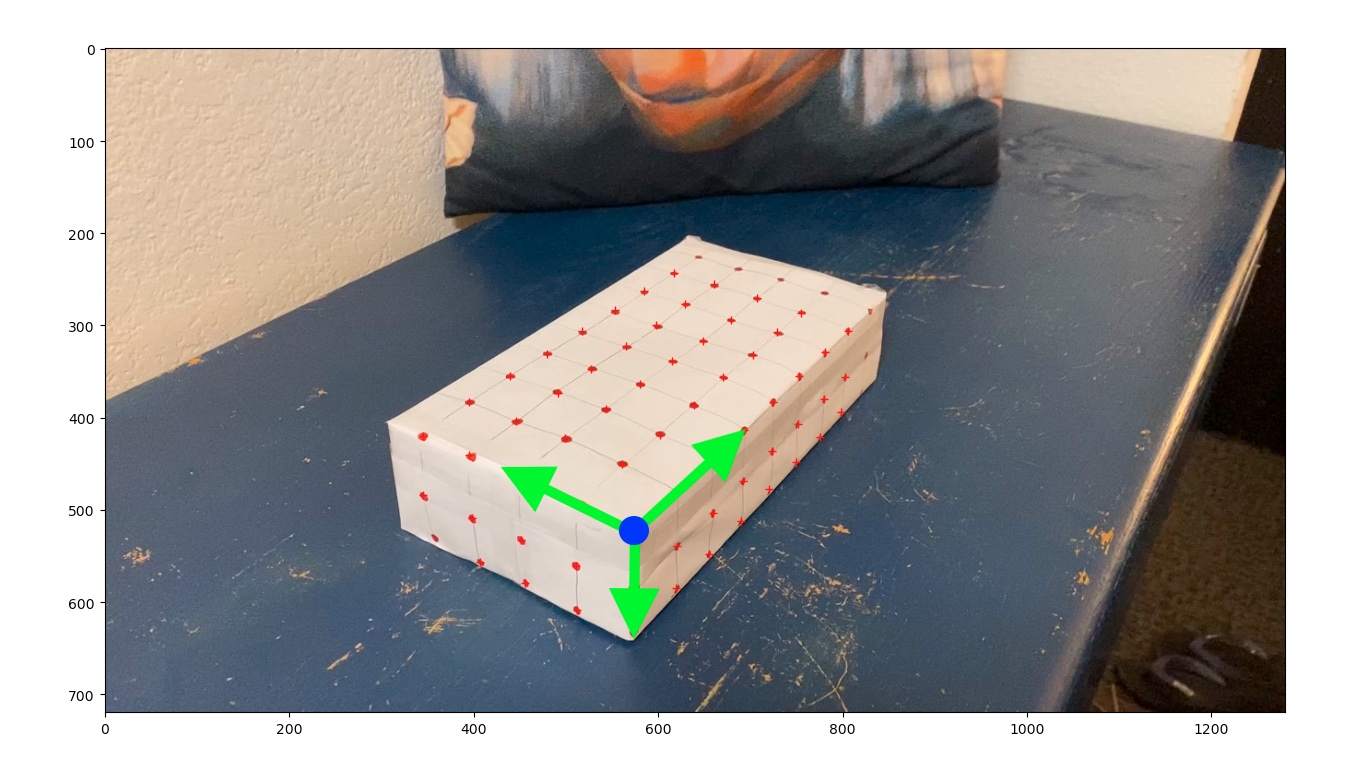
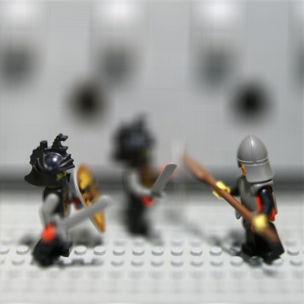
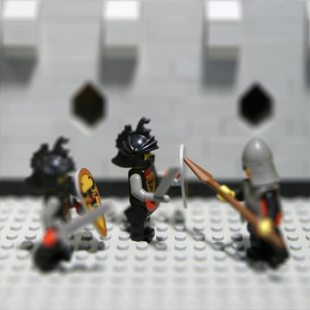
To ensure good tracking, I filmed a box with a grid of evenly spaced points as the real-life scene to place my 3D objects. I selected the starting locations of the grid points, which would later be used to initialize the tracker. I also defined 3D locations for these points relative to the coordinate system shown below, with the origin at the corner of the box.
Propagating Keypoints with Tracking
With the correspondences defined for the first frame of the video, I then used the MedianFlow tracking algorithm to locate where the dots on the box moved over time. A unique tracker was assigned to a each dot, meaning that the correspondence to its 3D position was preserved over time. The tracker I used was based on similarities inside a bounding box across neighboring frames, with the center of these bounding boxes tracking the actual dots. The bounding boxes started with a size of 8x8 pixels, but this size could change over time. I found that the camera calibration worked better if I rejected tracked points whose bounding boxes had inflated to a size greater than 16x16, since this seemed to indicate uncertainty by the tracker.
Camera Calibration and Cube Projection
Using the tracked 2D dot positions and their corresponding 3D world locations, I computed the parameters of a homographic camera projection matrix for each frame. This type of 4x3 matrix, written below, describes how to convert a 3D position (represented as a 4D vector, padded with a 1 at the bottom to allow for translations) to a 2D position (also padded). The parameters of this matrix can be solved for using least squares.
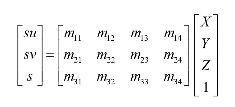
Finally, the camera projection matrix can be used to project virtual 3D points to the 2D image such that they appear to exist in the same scene. I projected a 2x2x2 cube onto my scene in this manner, first translating by 1 unit along the x and y axes, resulting in the video below!
PROJECT 2: LIGHT FIELD CAMERA
Summary
For my second project, I chose to implement depth-of-field (DOF) refocusing and aperture adjustment using light field data. This data comes in the form of multiple images captured from the gridpoints of a camera array which is orthogonal to the optical axis. The particular source I used for these sets of images was the Stanford Light Field Archive. The visual effects are implemented through selection, shifting, averaging of the individual images. This project made me think differently about how cameras (and our eyes) collect light to produce images that portray depth.
Depth Refocusing
This effect was achieved by averaging all of the images in a 17x17 grid, each shifted by some amount. This amount was based on the position of a camera relative to the center of the grid -- the camera at position (8,8) -- and a parameter alpha which effectively controlled the focus plane of the resulting image by uniformly scaling the offsets of each image. A positive alpha meant that the images were shifted outwards from their original position, resulting in a focus plane far away, while a negative alpha meant that the images were shifted inward, resulting in a focus plane close to the camera(s). This works due to parallax, which means that when a camera moves, objects close to the camera move farther (in the 2d camera projection) than faraway objects.