CS 194-26 Final Project
By Sriharsha Guduguntla
Project 6 entails doing two different projects in one. I did the Image Quilting Project and the Image Light Field Camera Project. I also did the Bells and Whistles for the Lightfield project. You can click on the links in this description to scroll to the associated project.
Image Quilting
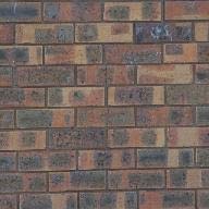
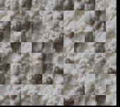
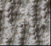
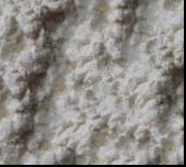
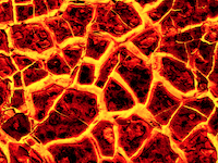
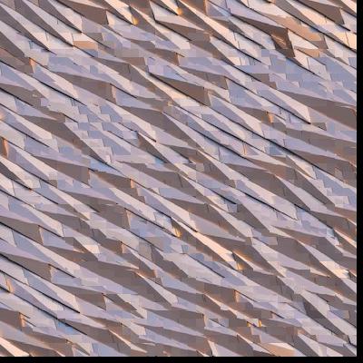
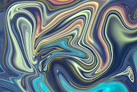
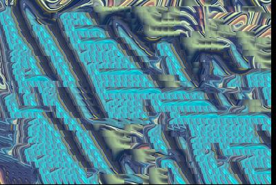
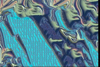
For this project, I implemented the texture transfer technique presented in Prof. Efros's SIGGRAPH 2001 paper. I took several intermediate steps to get to the final transfer stage. The steps are:
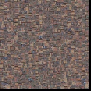
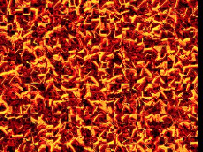
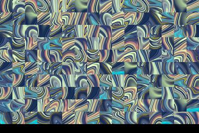
- I randomly sampled the inputted texture into square samples of a fixed size and just randomly stitched all the images together to make a very simple, low-effort expansion of the texture.
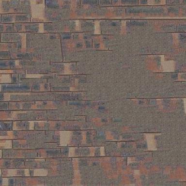
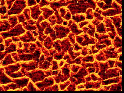
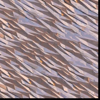
- Seeing that the random sampling was very choppy and not clean, I implemented the second part of the spec which was to start with a random patch at the top left and then for every new patch being sampled, choose the sample patch that would result in the minimum overlapping SSD cost and overlap over the left and top of the image with the output.
- Seeing that the random sampling was very choppy and not clean, I implemented the second part
of the spec which was to start with a random patch at the top left and then for every new
patch being sampled, choose the sample patch that would result in the minimum overlapping
SSD cost with the output's overlapping portions. When choosing the
patches with min SSD, I sampled the k-smallest SSD patches and chose a random one out of the
k patches. k is another parameter inputted as
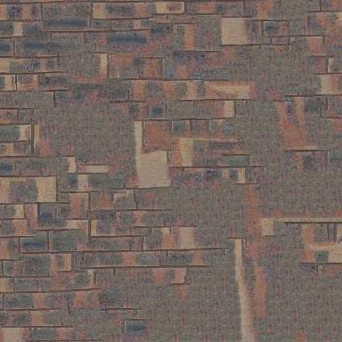
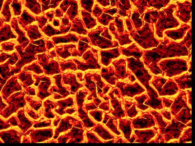
tolin my implementation. - After the last step, it wasn't as patchy, but there were still vertical and horizontal lines visible between the patches making it still not very smooth. To fix this, I implemented seam finding which involves calculating a cost image which is basically a matrix where each pixel represents the SSD cost of the patch centered at that pixel and the output overlap. After the cost image is computed, then a min cut algorithm is used to find the minimum cost path through the cost image allowing us to find a non-linear divider through the overlaps. This allows for the linear horizontal and vertical lines to be gone and the connections between patches are a lot smoother and accurate.
| Original | Random | Simple Overlapping | Min Cut/Seam Finding |
|---|---|---|---|
 |
 |
 |
 |
 |
 |
 |
 |
 |
 |
 |
 |
 |
 |
 |
 |
 |
 |
 |
 |
Seam Finding
For the following picture, here is an illustration of the seam after finding the min cost path through the cost image.
Left Overlapping Patch of Sampled Patch
Left Overlapping Patch of Result Patch
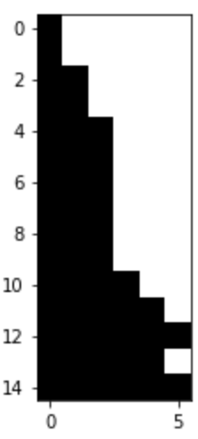
Cut Mask
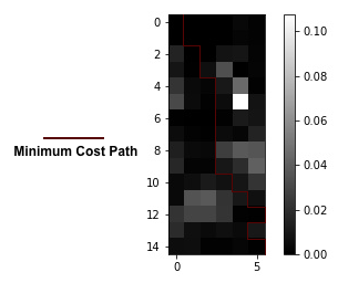
SSD of RGB values of overlapping patches (bndcost) with min cost path seam drawn in maroon
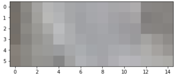
Top Overlapping Patch of Sampled Patch
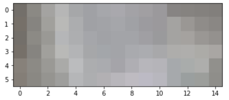
Top Overlapping Patch of Result Patch
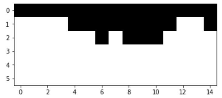
Cut Mask
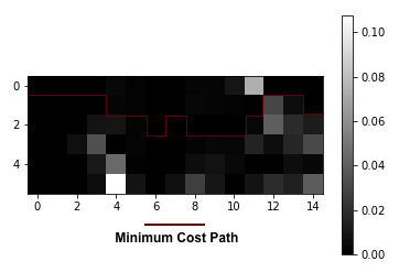
SSD of RGB values of overlapping patches (bndcost) with min cost path seam drawn in maroon
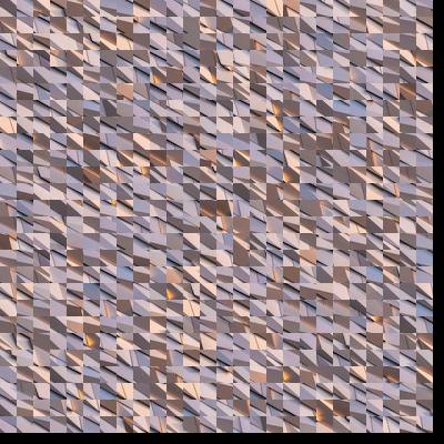
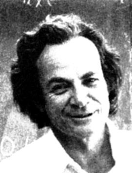
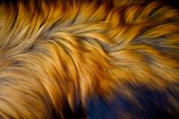
Texture Transfer
The texture transfer works by taking into account the new transfer image that is
inputted and at each instance when it decides to choose a patch, it calculates a weighted sum of the
SSD instead using a parameter called alpha which controls how prevalent the image
should be in
the texture. This image works as a guidance image for the patches to be put together in such a way
that the patches in the transfer image that correspond best to a certain sampled patch will let us
know that the sampled patch should be included.
| Texture | Guidance Image | Result |
|---|---|---|
|
 |
|
 |
 |
 |
While implementing this, I faced many challenges, particularly around small bugs here and there and learning how to properly visually debug. Moreover, a lot of times, my code took a long time to run which made it more difficult to quickly test changes. From a design perspective, I also found it a little hard to organize my code because there were so many moving parts. And something I didn't consider the whole time was that the images passed in could be any size and don't necessarily have to be the same size. As a result, I had to go back and add extra cases to handle these edge cases so that the image sizes don't really matter. I also found this project challenging, but rewarding in general because the final results are quite cool and worth the time that I put in because I learned a lot through the process, even stuff that I didn't learn all semester so far.
Lightfield Camera
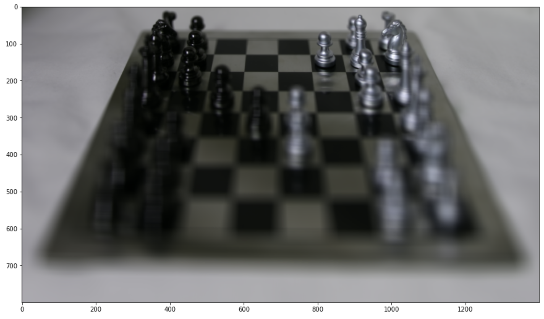
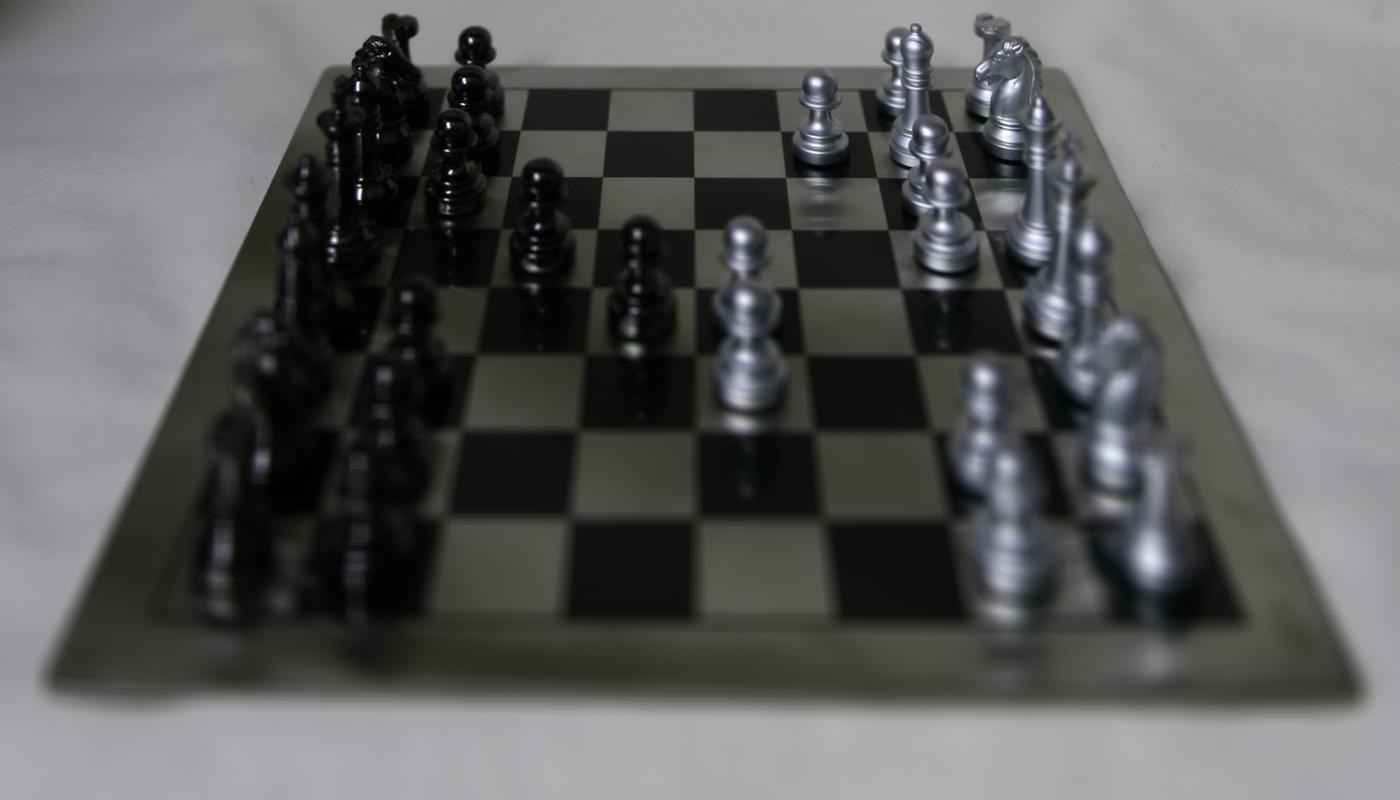
This project has two different parts, one where you mimic adjusting the focus of the
image by making it focus closer towards the front of the image versus the back. This is called depth
refocusing. The second part of the project involves mimicing the adjustment of aperture by averaging
fewer or more images that are within a radius of a fixed focus point in the image. To do this, I
first used a dataset from Stanford Lightfield Archive where they setup a 17 x 17 grid of equally
spaced cameras that took pictures of the same image (chess board) at the same angle, but just
off-centered. Each of the coordinates for these cameras is a set of (u, v) coordinates.
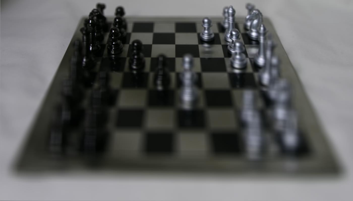
I first naively
averaged all the
images to get an mean image where only the back part of the image is in focus (as shown below).
Part 1: Depth Refocusing
For Part 1: Depth Refocusing, my
approach was to obtain the (u, v) coordinates of the input images (which I parsed
from the
filenames
of
the chess dataset from
Stanford
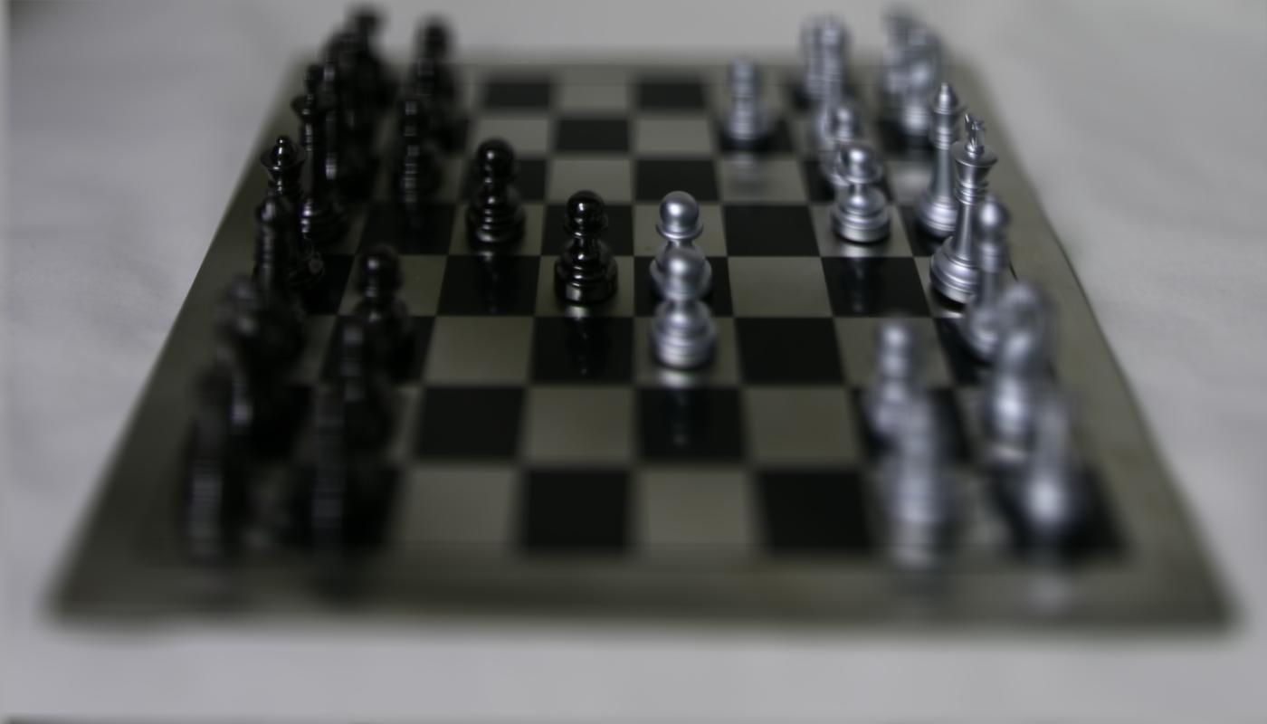
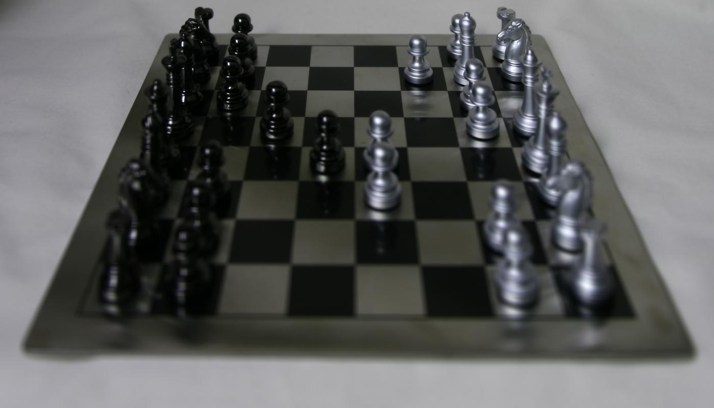
Lightfield Archive). Then, I chose the image at the center of the grid at coordinates
(8, 8). Then, I looped through all the images and shifted them closer to the center
image by shifting them by (alpha * (8 - u'), alpha * (v' - 8)) where (u',
v') are the
coordinates of each image and alpha is a constant scaling factor between [-1, 3) and
0.2 increments
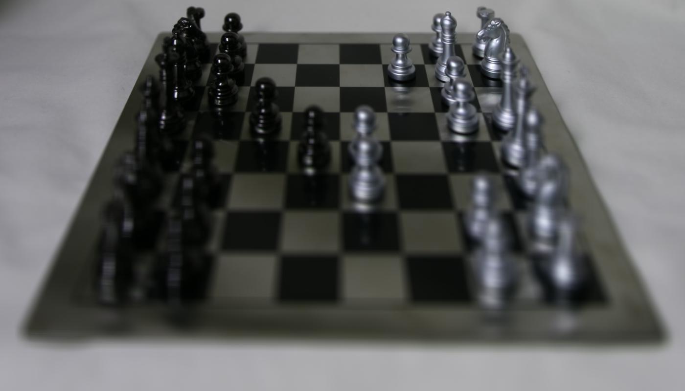
that allows us to switch the focus of the image from the back to the front incrementally. Here
is a gif as well as some frames with different alphas. As alpha increases, the focus switches to
the front of the image.
alpha = -1
alpha = 0.2
alpha = 1

alpha = 1.8
alpha = 2.8
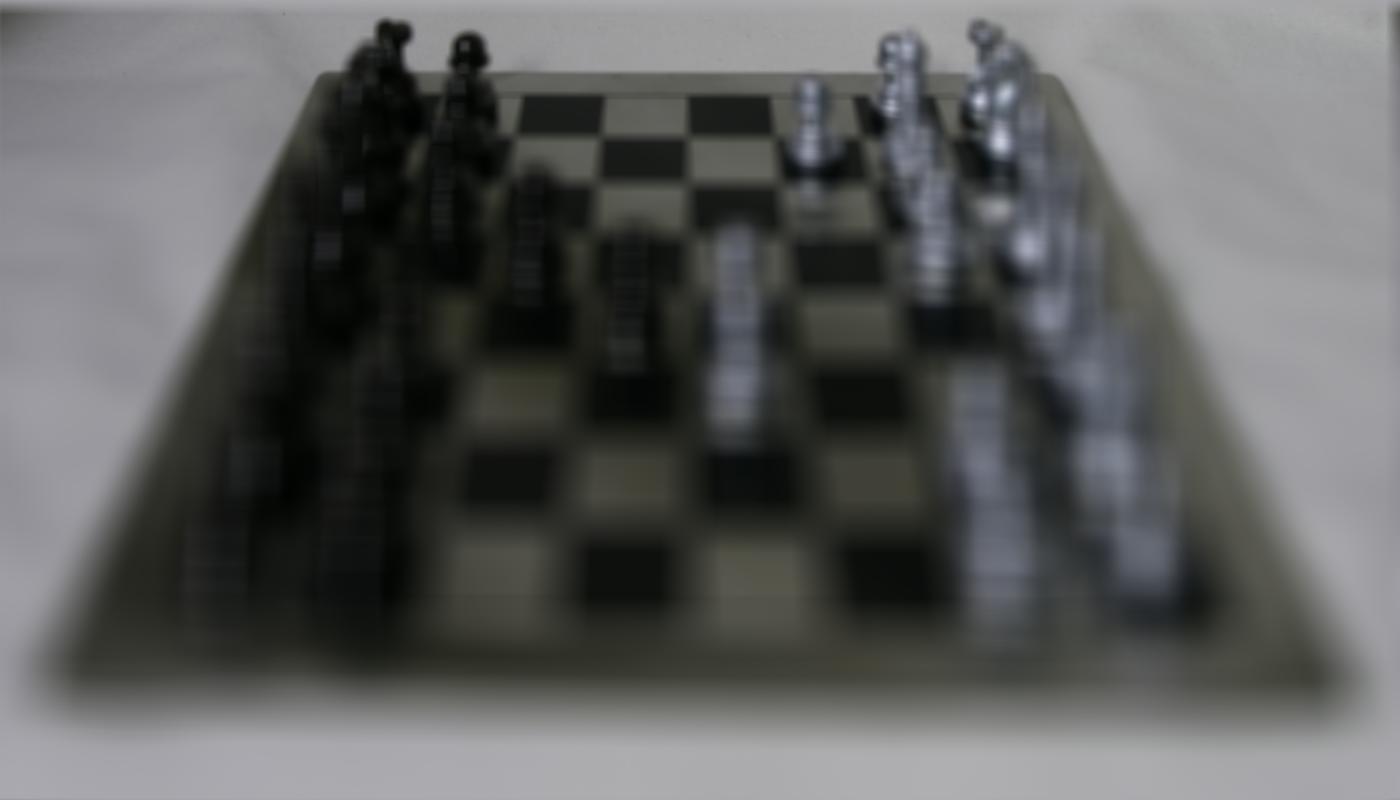
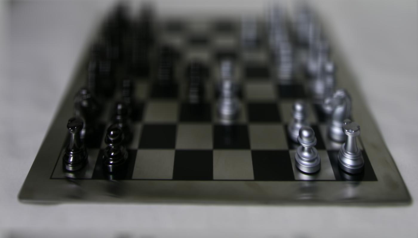
Part 2: Aperture Adjustment
For Part 2: Aperture Adjustment, I chose the image at the center of
the grid at coordinates
(8, 8). Then, I took in an input radius value and selected all images
that were radius away from the center point. For larger values of radius, this mimics a larger
aperture. Then, I averaged the selected images. Therefore, as radius increases, I average more
and more images that are in the vicinity of the center point. Therefore, as the radius increases,
more and more light "enters" the camera causing more of the surroundings to get blurred. Radius goes
from [1, 6) in the gif below.


radius = 1
radius = 2
radius = 3
radius = 4

radius = 5
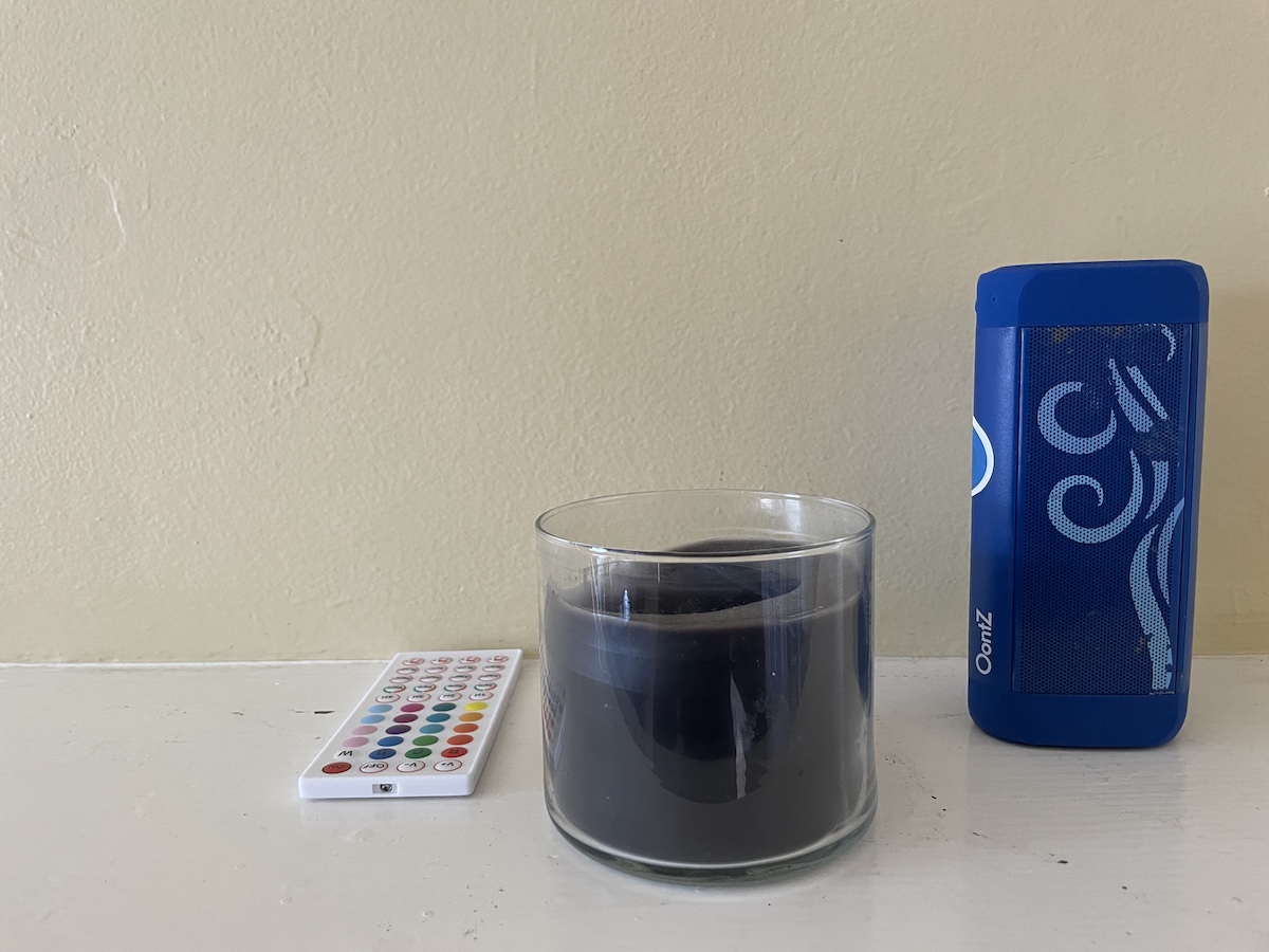
Bells and Whistles
For the bells and whistles for this project, I decided to try taking my own pictures with my phone to
similar to the Stanford Lightfield datasets. However, instead of having to take 17 x 17 = 289
pictures, I decided to use a smaller grid of 5 x 5 = 25 images. Here is the base image of a candle,
speaker, and remote in my room. Unfortunately, the results were not very good at all because of the
way I likely took the pictures. I did not have access to a precise lightfield camera like the
Stanford dataset, so it was harder to keep track of exactly where my phone should be placed in the
grid. This was likely the reason for the very unusual results below.
Depth Refocusing (alpha goes from [-1, 3) with 0.2 increments)
Aperture Adjustment (radius goes from [1, 6) with 0.2 increments)
What I learned about Lightfields
I learned that lightfields can be very powerful and even without an actual camera adjusting its aperture and focus, it is still possible to manipulate images given a proper set of lightfield data. I also learned that in order to get proper results, precise equipment that can capture lightfield data like Stanford's 100 VGA video cameras are needed. Otherwise, it is very difficult to take pictures with a handheld device like a phone to mimic the lightfield datasets.