Overview

In this project, I created visual effects that can be done with a light field camera through simple operations of light field data. I implemented depth refocusing by shifting the pictures by a specific amount, and I implemented aperture adjustment by using a subset of the total pictures.

Depth Refocusing

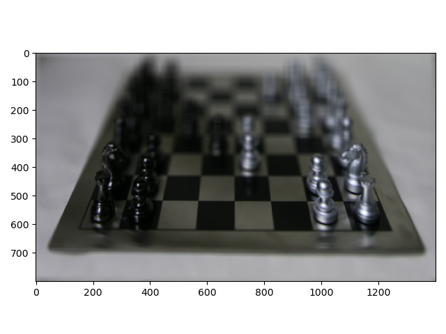
To do depth refocusing, we shift the images based on their distance from the center image. Since there are 17x17 images, the center image is the one at (8, 8). For all of the images (x, y), we shift them based on the equation C*((x, y) - (8, 8)). We subtract their positions from each other, which we get from the image name. We then multiply it by a constant to see how much we shift. The more we shift, the clearer the objects at the front will be because their distance changes the most from camera to camera. Because the objects in the back do not vary in position as much from camera to camera, they will be more blurry as we shift images more since they will be more misaligned. Currently the image is focused on far away images, so by increasing C, we move the focus to the front.

The following image is the chess board when just averaging all of the pictures.

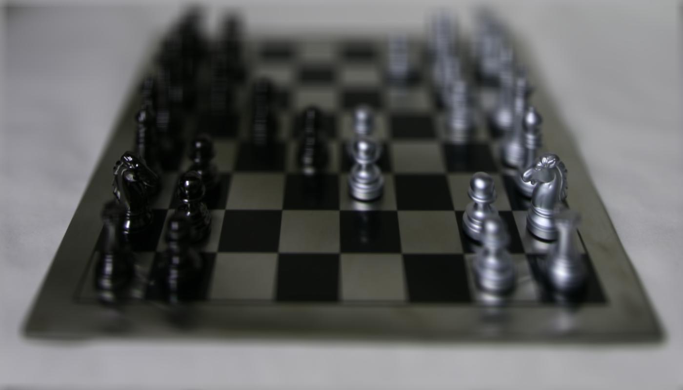
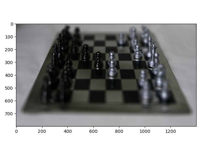
The following images are the chess board with different C values.

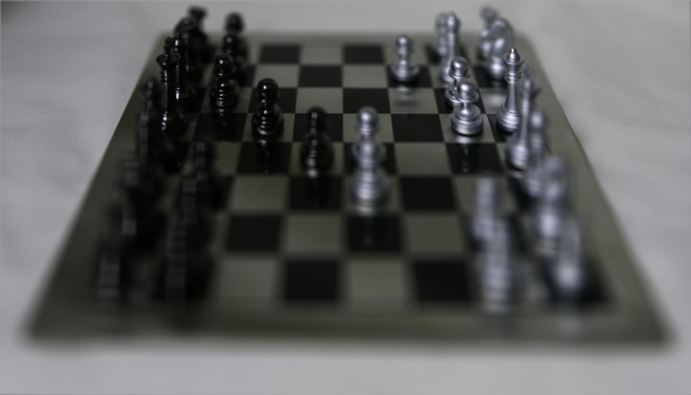
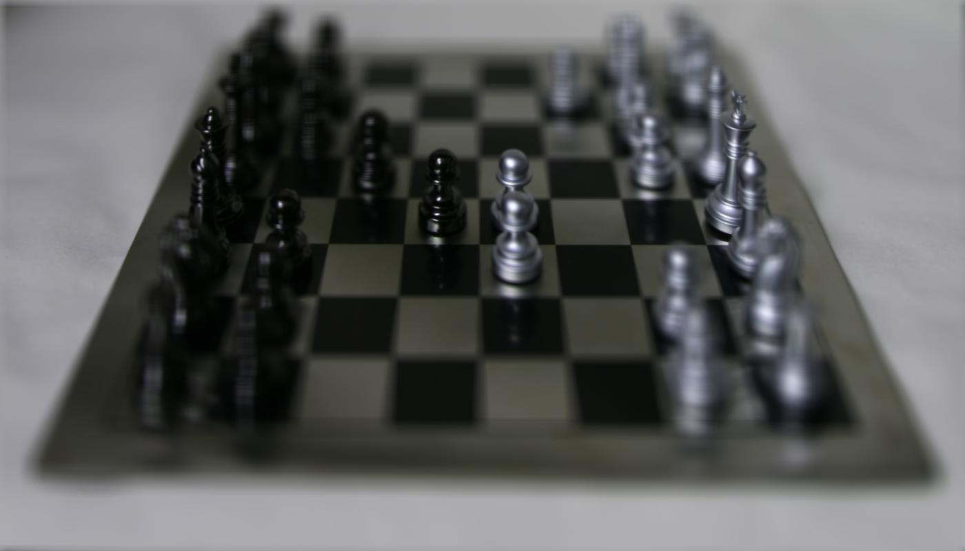
Here is the gif of the depth refocusing from C = 0 to 0.5.

Aperture Adjustment

To do aperture adjustment, I first used the depth refocusing to shift the image's focus to the center of the image. To change the aperture, we just take a subset of the images. I checked that the distance from center was less than a certain distance. So for an sub-image at (u,v), I checked if the L2 distance was less than R for a specific radius ((x - 8)^2 + (y - 8)^2 < R^2). This is how I get a subset of images around the center.

The gif below shows the aperture adjustment.

Bells & Whistles: Interactive Refocusing

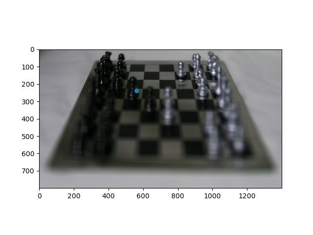
To do interactive refocusing, I combined the exhaustive search from project 1 and the calcualtion for the C value in this project. I first clicked on a specific spot on the picture to focus. To do this, I needed a patch around this point to be in focus. Therefore, I used a 60x60 pixel patch around this point and compared the (0, 0) subaperture picture with the center subaperture picture at (8, 8). I shifted the (0, 0) subaperture picture with exhaustive search to find where the patch around the chosen point has the smallest SSD. This is how much the picture needed to be shifted in terms of (s, t). I did exhaustive search from -20 to 20 pixels on both the vertical and horiztonal direction to find the best shift. We then can recalculate C with the equation C = s/(x - u), where s is the shift in the vertical direction, u is the vertical position of the (0, 0) image and x is the vertical position of the center image. We can also find it using C = t/(y - v), where t, u, and y are the same values in the horiztonal direction. However, these two values may not be the same due to rounding error, so to calulate the final value of C, I take the average of the two values: C = (s/(x - u) + t/(y - u))/2.

After finding the C value, we can now recreate the refocused image using the process found in depth refocusing section. Below are some examples with a chosing point (blue point) and the refocused image.

Summary

I found it really interesting how adding less of the images was able to change the aperture, and how just having these different images with their respective distances, we were able to make these different effects.

Overview

In this project, I used image quilting to create a larger texture image from a smaller image. We do this in multiple ways. First we just randomly stitch patches together. Next, we overlap patches by finding the patch with a low overlap SSD. Finally we implement seam finding to get a non-linear boundary. Finally, we use this to transfer texture to a different image.

Randomly Sampled Texture

For this, I randomly sampled a patch with patchsize, and I filled in the output image until I cannot fit anymore patches, leaving black borders on the edges if there is extra space. To sample a patch with patchsize, I randomly chose a top left corner and got the patch from there with patchsize.

Overlapping Patches

To implement overlapping patches, I first needed to implement SSD. This calculated the SSD of the overlapping part of the sample patch and the patch already chosen in the output image. I then implemented choose_sample, which randomly chooses a sample patch based on the SSD cost. We don't always want to choose the minimum cost, or else we just recreate the image, so we randomly choose and image where its cost is less than the minimum cost * (1 + tolerance). The tolerance I used was 0.2. Finally, to implement the main algorithm, for every patch we output, I calculated the SSD cost for every possible patch from the sample. I then used choose_sample to randomly choose one of the patches with a lower cost, and that patch is added to the final output image.

Seam Finding

To do seam finding, I wrote the cut function to find the minimum cost path from left to right of a patch based on the boundary cost. The cost is calculated by the SSD between the output patch and the sampled patch. I am finding the best path over where the two patches overlap. To do this, I used dynamic programming by finding the shortest path from left to right by checking i-1, i, and i+1 of the previous column and getting the smallest one. I keep track of the path that each row makes, and I find the minimum value on the right most column at the end. I then retrace its steps and this will be the minimum cost path. I then use this path to make a mask by having everything under the path be 1s and everything over be 0s. Finally, if the path overlaps on the left side and the top side, we take the intersection of those to get the new boundary.

Here is the sample that I used.

Below are images comparing all three methods.

Here are the steps for quilting together two images. Both images are 40x40 pixels, and they have a 10 pixel overlap.

From the images above, we see that we first calculate the SSD cost in the overlap patch. We then try to find the minimum cost path from the top to the bottom to find a good way to divide the overlap patch. We then have the left side of the divide be from one image and the right side be of the other image so we can have a clean divide as shown in the output.

Here are a few more examples of texture quilting.

Texture Transfer

Texture transfer was implemented by adding an extra cost to the texture quilting code. I blurred the texture as well as the image we are trying to transfer to. For every patch, we not only take account the SSD of the overlap section, we also find the SSD between the blurred texture and the blurred image patch at that section. We take the weighted average of these two values to get the new cost value. I put more weight on the difference between the image we're trying to make so we have the correct light intensities, so it looks similar to our target image.