Hi! Here is my two part final project for Computational Photography, exploring special topics presented in the course!

Part 1: Lightfield Cameras

Depth Refocusing

Aperture Adjustment

Summary

 

Project Part 2: Poor Man's Augmented Reality

Keypoints with known 3D world coordinates

Calibrating the Camera

Projecting a cube in the Scene

Let's get started!

Part 1: Lightfield Camera - Depth Refocusing and Aperture Adjustment with Light Field Data

With a conventional camera, we capture just the projection onto a single plane, resulting in 2D data, focused at a single depth of field. However, lightfield data is captured by inserting a 17x17 microlens before the sensor plane, resulting in 289 images that capture infomation about the structure of light in the world. Using computations of shifting and averaging, we can recover images focused at multiple depths of fields from just a single photograph. Because the aperture of the original photograph has a width 17x larger than the microlens' apertures, even a short exposure can capture images with high SNR.

The lightfield data I use in my implementation is from The Stanford Light Field Archive, and uses the approach that is outlined in this paper by Ng et al.

A) Depth Refocusing

Lightfield data is from multiple images from different angles, and we know that these shifts cause images closer to the camera to shift more than the ones that are far away. However, if we first shift these images to bring closer items back in focus, we can effectively change the depth of field. The shift is determined by the distance between the u-v image plane location of each microlens image compared to the u-v location of the center image, scaled by a factor, proportional to the depth of field.

So, I first obtaining the center image (I used the image for the lens at 8, 8). We then compute the displacement from the center location using the recorded u, v coordinates for each image. We can select a depth of field and shift each image by its displacement from the center scaled by the depth value. By averaging these images, we can obtain an image focused at the chosen depth of field. Below is two examples of varying depth refocusing of a lightfield camera image.

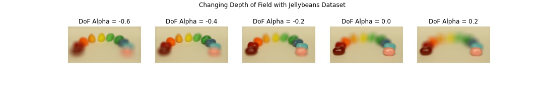
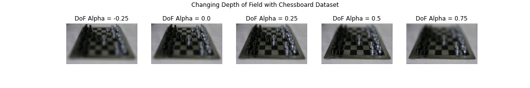
The gifs below displays a varying alpha. For the chessboard, we vary from -0.8 to 0.5, and for the jellybeans, from -0.6 to 0.4. The reason for the different ranges is due to different initial focuses in the image-- the chessboard had a focus in the back, and the jellybeans in the front.

 

B) Aperture Adjustment

When we take a single lightfield camera image, it is almost like a pinhole camera image. While it has an identical aperture to the larger camera, the aperture width is much smaller (in our case, 17x smaller). This smaller aperture size allows the lens to block rays from multiple angles, creating a sharper image. Additionally, when the image rays are perpendicular to the optical axis, they are less blurry because multiple rays don't scatter. On the other hand, objects coming from angles to the optical axis appear blurrier because they end up furter from each other on the sensor plane.

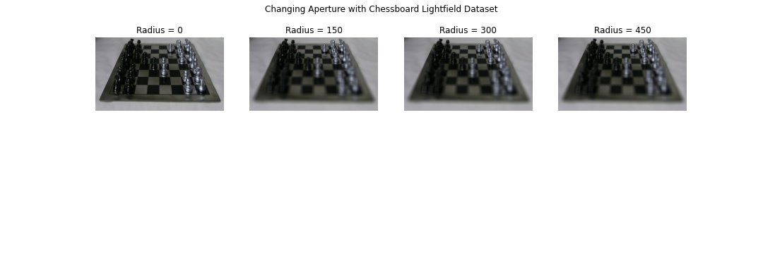
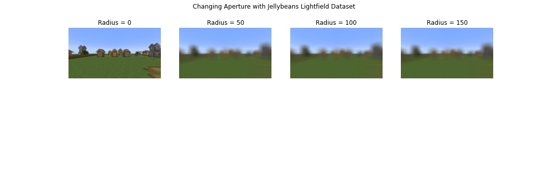
We can use a lightfield camera to simulate a larger aperture. To do this, we specify a radius about the center point. Only images that fall within that radius will be included in the average. As we increase the radius, this will create a focus around that center point focus (the region that was perpendicular to the optical axis) and blur the perimeter, simulating decreasing the f-stop or increasing the aperture.

Below are examples of what this looks like!

And a gif of the chessboard:

 

C) Bells and Whistles: Implementing on my Own Data

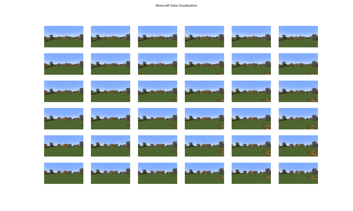
In this next part, I attempted using my own data! I didn't have fast access to a 3D printer to simulate a microlens grid, so instead I called on my brother (shoutout to Srihan Basvapatri!) to help me capture photographs within a video game. We decided to capture movement along a 6x6 grid in Minecraft, and the source images are shown below.

Here is the video result of the final gif refocusing depth.

I think this worked so well because the movements along the grid were incredibly precise. I also learned that I could have simply used the microlens grid coordinates rather than the image coordinates for my refocusing and aperture adjustment procedures.

The results varying aperture didn't work as well, but I think this might be because I adjusted the radius too quickly.

 

D) Summary and Takeaways

In implementing this project, I learned how simple lightfield computations can be. However, my computations and downloads were slow, and lightfield cameras significantly limit the resolution of images. Given these storage, computation, space, and cost constraints, I think we're still quite limited from making lightfield cameras widely available, however, they would be a blessing for when my photos just don't seem exactly focused.

Part 2: Poor Man's Augmented Reality

For my second project, I experimented with implementing an AR system with a very simple setup. Starting with a box with grid labels, I tracked points between image frames using corner detection techniques from earlier in the semester and inserted an object into the video.

I first started by tracking inputted points between the very first frame and the second frame. This was done using a plt.ginput function, and made us of Harris Corner Detection like in Project 4 to detect the corners within the second image. From there, I found the corner points that were closest to my hand-labelled points from the first frame. Repeating this over all video frames allowed me to propagate the same points throughout the video. This approach rests under the assumption that points don't move much in between frames.

From there, I found the camera calibration matrix that defined the system by setting up a system of equations. Unlike in Project 4, we know have 11 degrees of freedom instead of just 8. However, this isn't an issue because we've defined our world coordinate frame simply on the box, and we can choose an origin point from which to label the remaining points. After finding the transformation between the world points to the image points in the first frame, I was able to draw a box on the first frame. Then, by finding a new calibration matrix for every frame, I could similarly have this box, stationary in our world frame, move with the video frames. Below is the result of this!

Finally, I'd like to close with a huge thank you. I've really enjoyed this class and this semester, and being able to complete these cool projects also showed me how much I've learned! Thank you so much!