|
By Ana Cismaru and Prangan Tooteja
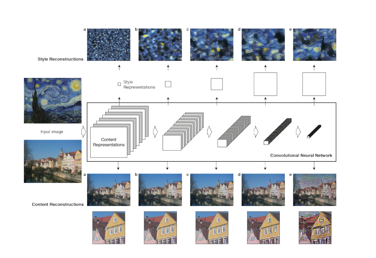
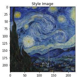
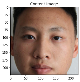
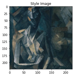
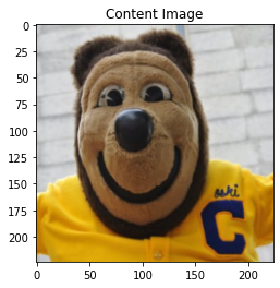
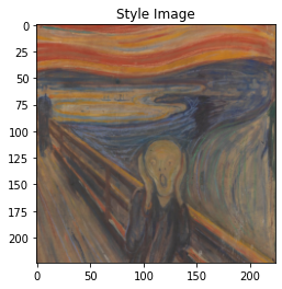
The first project we chose was to reimplement the paper "A Neural Algorithm of Artistic Style" by Gatys et al. The goal of this paper was to apply the style of an image A to the content of an image B. The network we used to learn style transfer used a pretrained VGG 19 network as a backbone but unlike a simple VGG network we followed the paper's advice and used an average pool operation insead of maxpool; and we used two more complex losses to capture the style and content of our inputs.
As shown in the graphic below, we can specify what layers we want to learn style from and what layers we want to learn content from. In our higher level layers, our content is more detailed. Additionally, depending on what layers we choose to capture style, we can capture more granular details or bigger/less specific shapes. Since we want to capture the complexity of the style, we use multiple layers (up to 16) to capture style, which specifying only one layer (layer 3 in our case) to capture content.
|
|
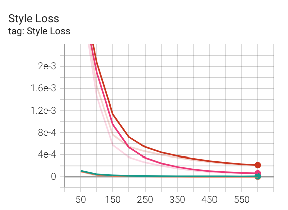
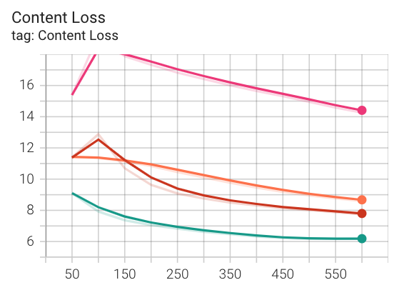
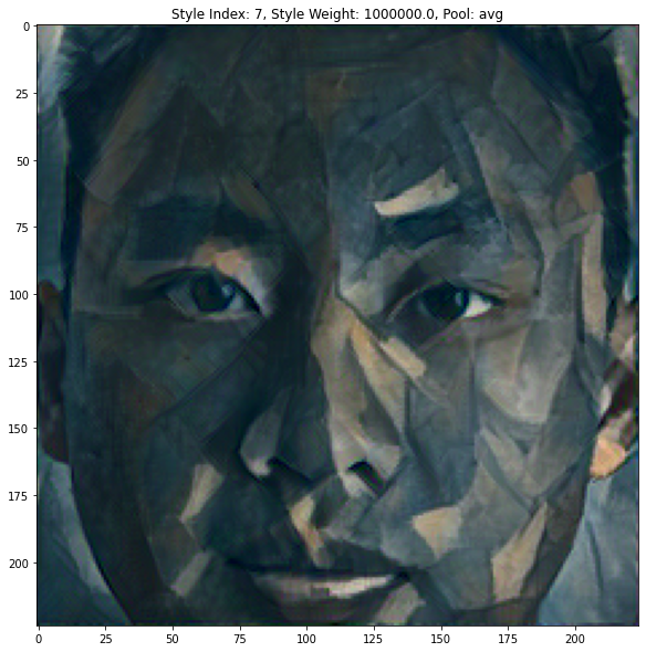
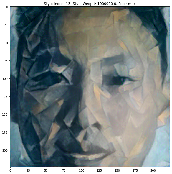
While training the model, we can visulize its style and content loss to ensure that it is indeed decreasing (ie: the model is learning its task correctly). We can also set up a hyperparameter tuning to explore which style layers yield the best results, how we should weigh style vs content losses, and whether using maxpool or avgpool works better. Below are some of our loss graphs. The red and pink lines represent hyperparameter setups using a network with max pool while the other two lines represent networks using avg pool. Like that, we can clearly see that avg pool performs better style-wise than max-pool.
|
|
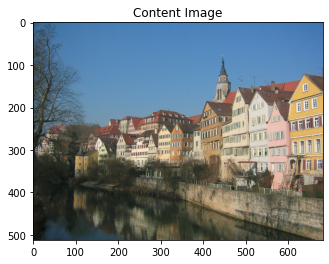
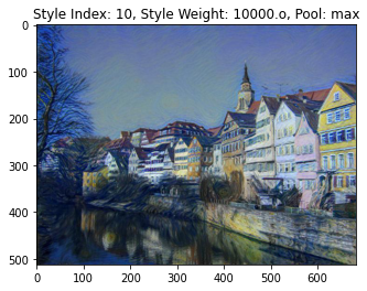
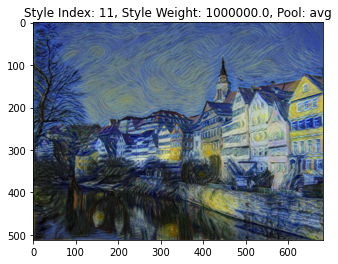
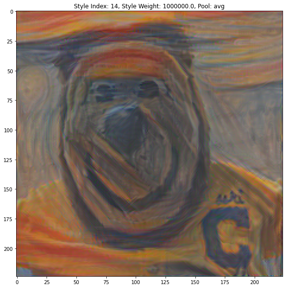
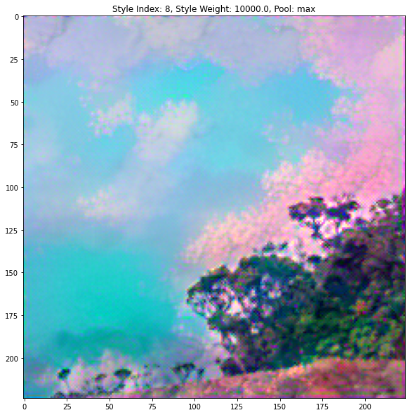
When it comes to tasks such as style transfer, inspecting losses proves to be insufficient to determining which set of hyperparameters works best. Instead, we found that visualizing our outputs proved to be much more informative as style transfer is a semi-subjective task. Below are some examples of our outputs with different hyperparameters.
|
|
|
|
|
|
|
|
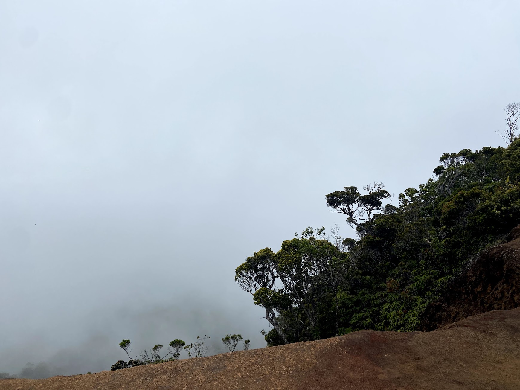
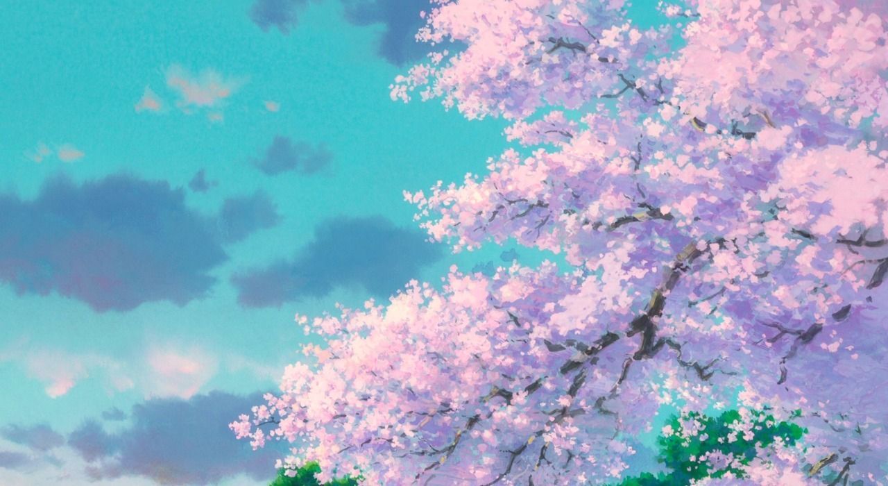
Here are more outputs with different content and different styles.
|
|
|
|
|
|
Our biggest takeaway from this project was the impact of choosing which layers learn style and content. It was super cool to see how one layer could learn both style and content at the same time. Additionally, this project helped me visualize how the depth of a layer can impact the information it learns from its input; we didn't get the chance to explore that too much in project 5 so it was fun to experiment with learning style at deeper or shallower layers.
For our second project, we chose to recreate "Image Quilting for Texture Synthesis and Transfer" by Efros and Freeman. This paper had two goals: the first was to synthesize more texture given an input texture and the second was to transfer texture to another image.
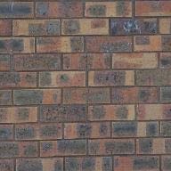
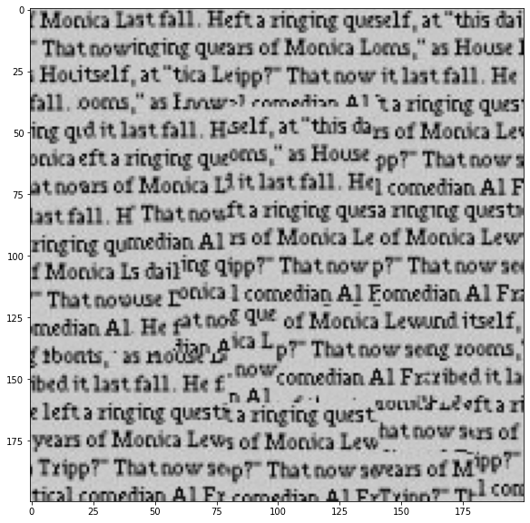
We first started generating more texture from an input using a very basic technique: randomly sampling patches from the input texture and placing them side by side in an output image. Of course, as seen below, these results were less than ideal as the texture is incoherant and we are very easily able to notice the presence of patches in our output image.
|
|
|
|

|
|
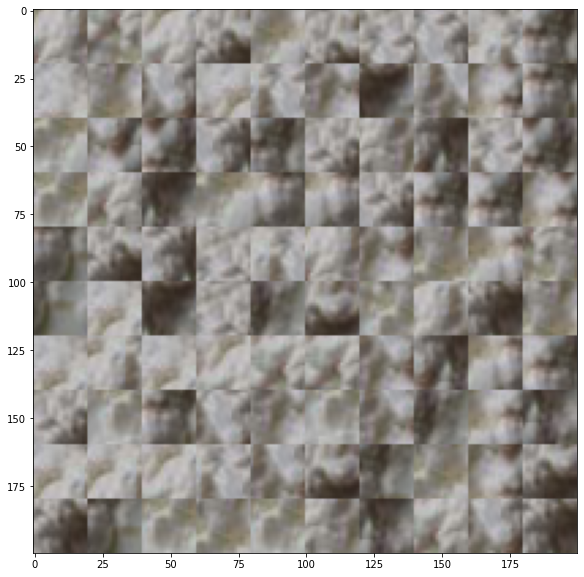
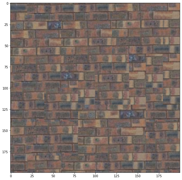
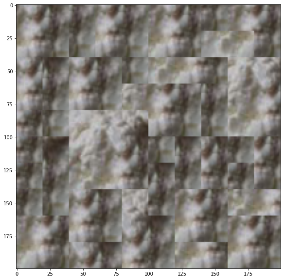
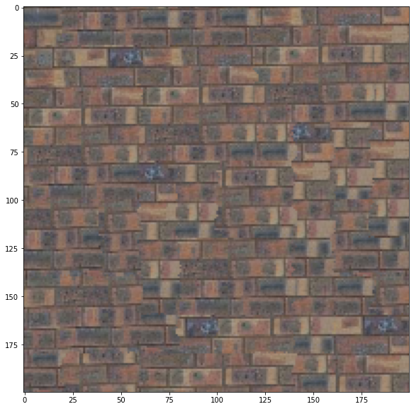
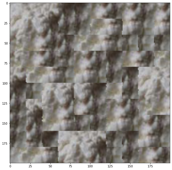
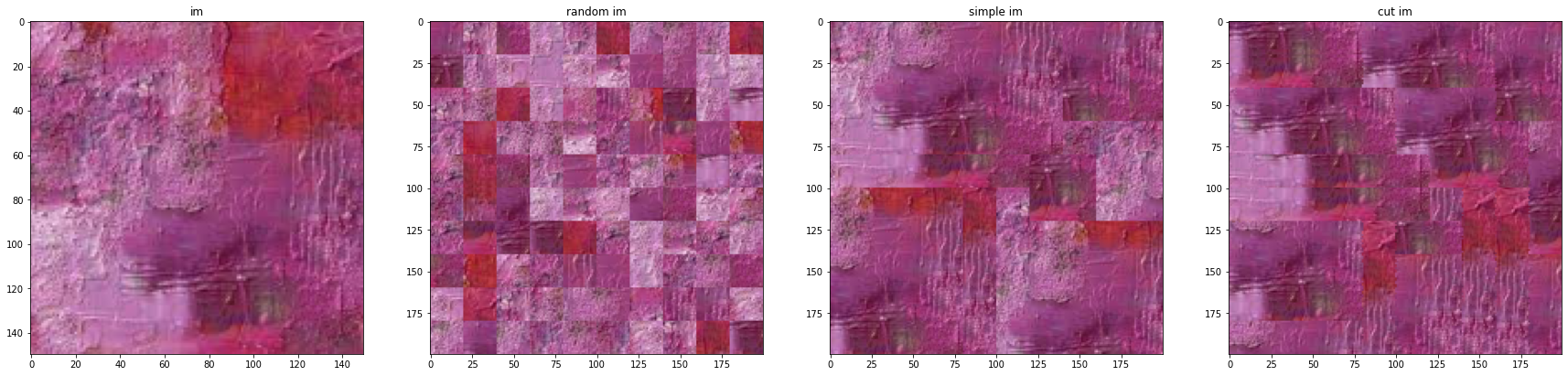
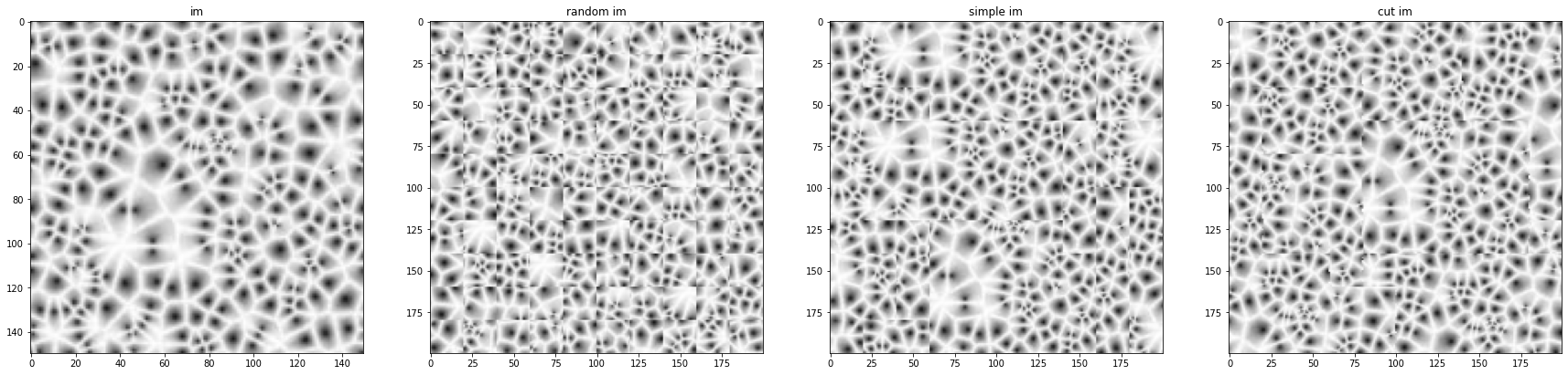
We then moved on to implement a slightly more complex technique called image quilting. The premise of this technique is that when choosing the next patch to place onto our outputs, we would select a patch from a set of patches whose edges match the edges of the patches already in the output image with whom it is neighbors. To determine which patches match best, we compare the regions of overlap between the new patch and existing neighbor using the SSD metric. One design challenge was figuring out how to consider overlap when dealing with patches that have neighbors above and to the left of them. For the horizontal and vertical edges, overlap regions were selfexplanatory, however we were also interested in having consistency between the diagonal neighbor in the top-left corner and the new patch. To achieve that, we also looked at a small overlap section between the diagonal parent and the new patch. As specified in the paper, we used a region of overlap that was 1/6 of the patchsize. We then select from all patches whose SSD is below a certain threshold. Like so we can ensure better consistency between patches in our output but we can still see the different patches as there are weird horizontal and vertical lines in our output. Below are some examples of outputs generated using this simple image quilting technique.
|
|
|
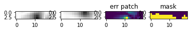
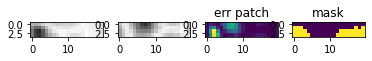
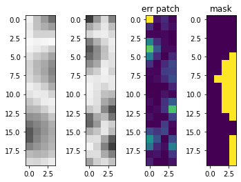
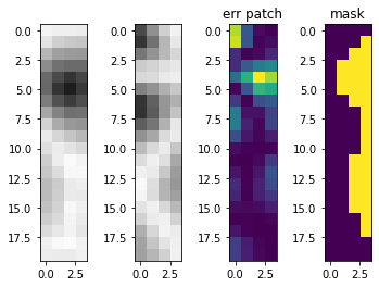
The issue with our simple quilting technique is that we are assuming that a straight line cut connecting neighboring patches A and B is the optimal cut. In fact, that is not the case hence us seeing horizontal and vertical lines between our patches in the output. To address this issue, we implemented a Minimum Error Boundary Cut function after identifying the best possible neighboring patch. The Minimum Error Boundary Cut uses dynamic programming to find the lowest cost path in our overlapping region. Below are some examples of the minimum boundary cuts along with the error of the overlap region.
|
|
|
|
With this, we can again see that our results are improved and the horizontal and vertical lines we were previously seeing have mostly disappeared.
|
|
|
We also ran the seam finding algorithm using our own data. Below are the results.
|
|
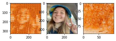
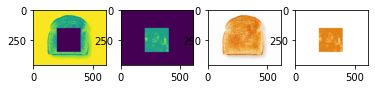
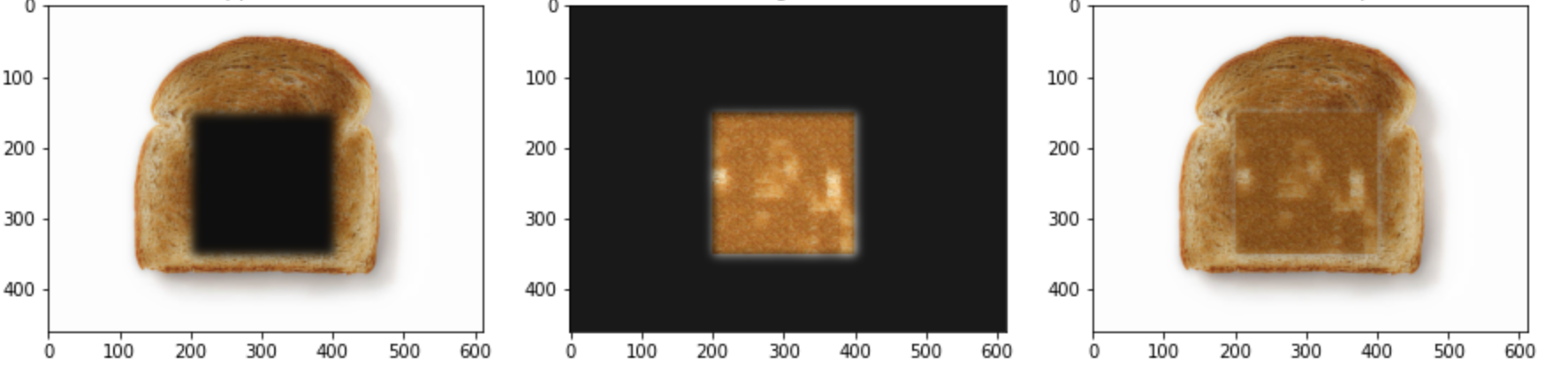
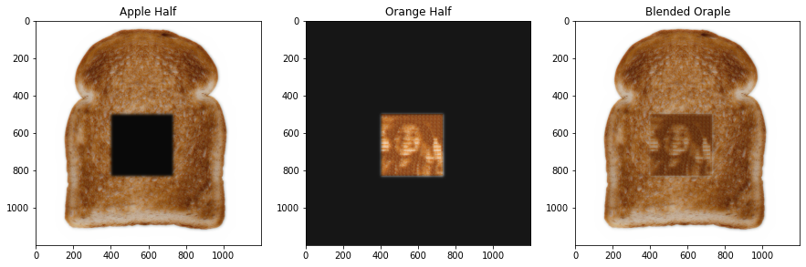
With our Image Quilting method setup we can also do other fun transformations regarding texture. For example, we can take some texture as well as a target image and we can apply that texture to the target image to make the target image look like it's made of that texture. The way we achieve this is by adding an additional cost term when selecting potential patches to add onto the existing output. The cost term is used to ensure that the content of the texture patch matches the content of the target patch it is attempting to replicate. To analyse how well the two patches are matching, we look at the SSD of the luminance of both patches (ie the grayscale version of the patches). Like so, we ensure that content is similar between the two and are able to recreate the target image using the texture input. Below are some examples of texture transfer.
|
|
|
Our biggest takeaway from this project is the power of simplicity. It was super awesome to see how such simple methods could generate such fun and complex results. We would be interested in seeing how methods like these compare to more recent methods such as GANs.
With our new texture transfer method, we can create fun artworks such as a toast with an outline of a face in it. To achieve this result, we first create a face with toast texture (see output above) and then used Laplacian Blending to insert the toast-face into a larger image of a toast. Below are two examples of toast in faces with different toast image sizes/patch sizes. It was slightly challenging getting the toast features to encapsulate such a detailed photo while also mainting the aspect of toast. With smaller patchsizes we could have a more detailed output but we lose the air pockets from the toast texture.
|
|
|
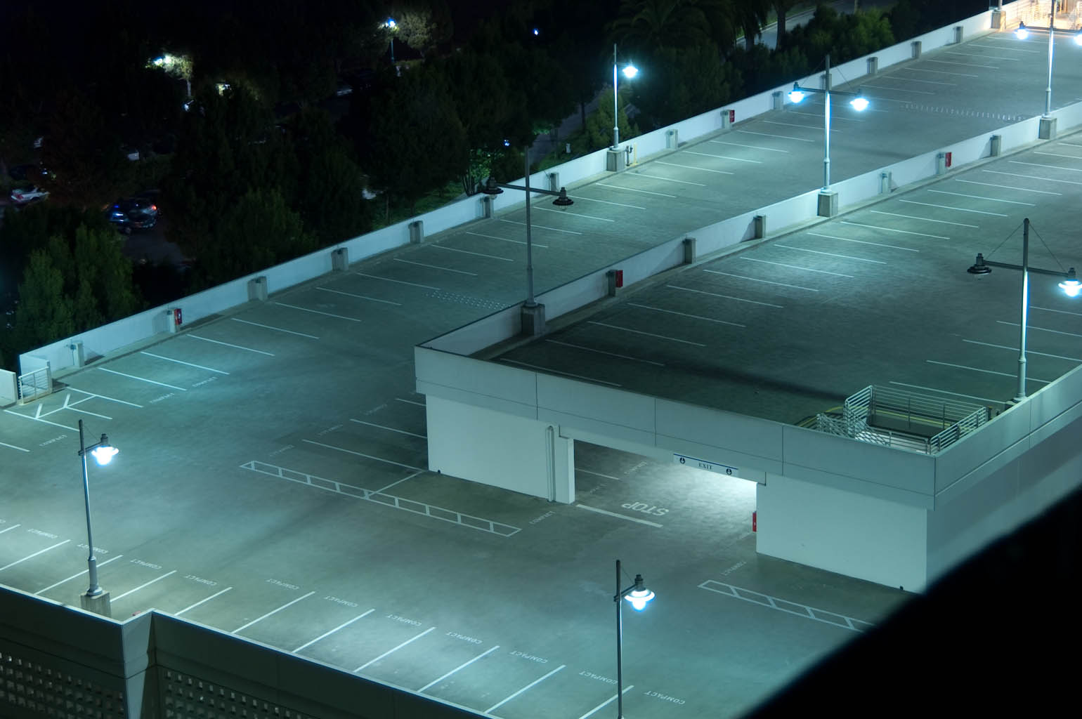
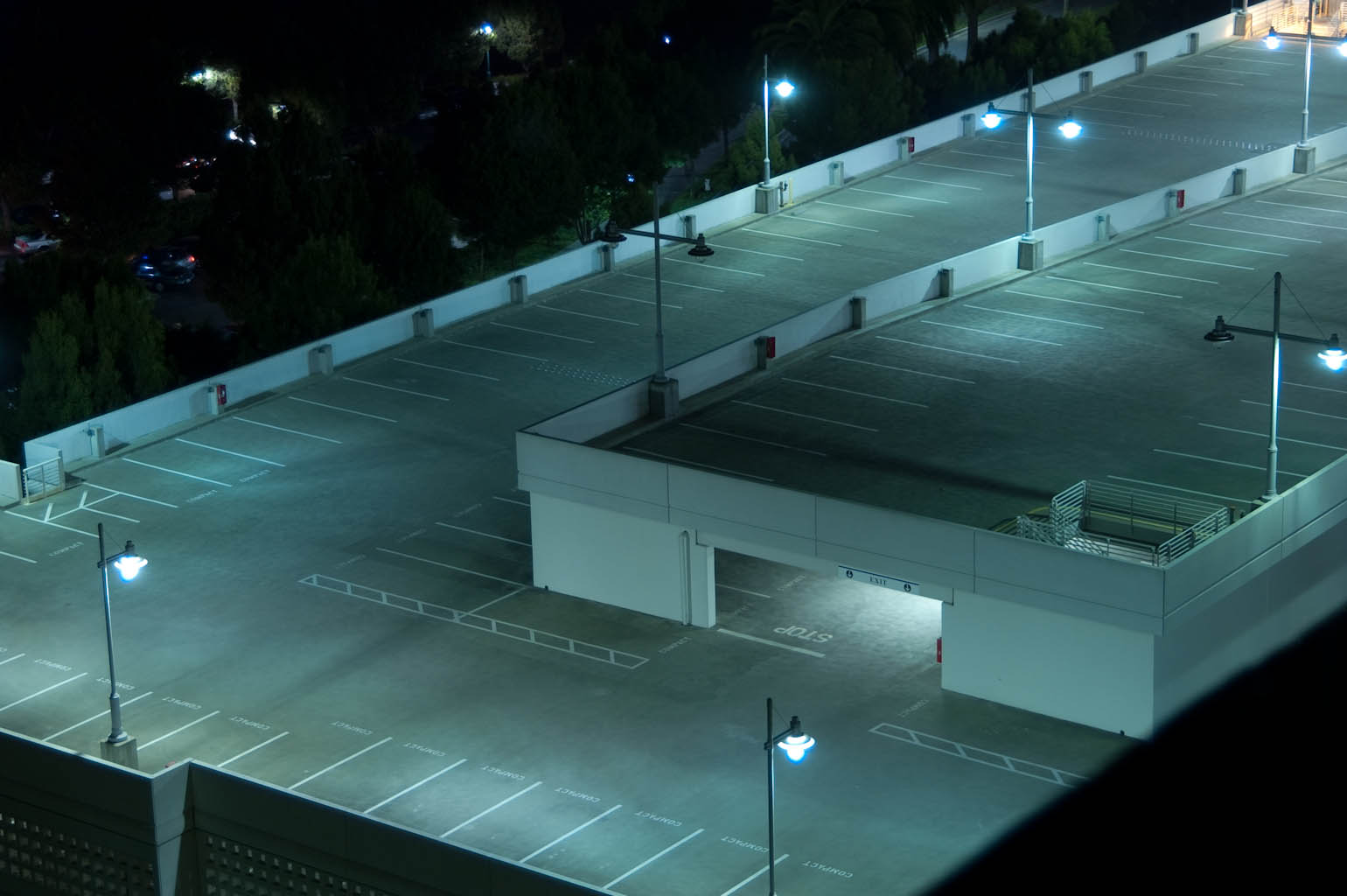
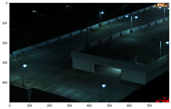
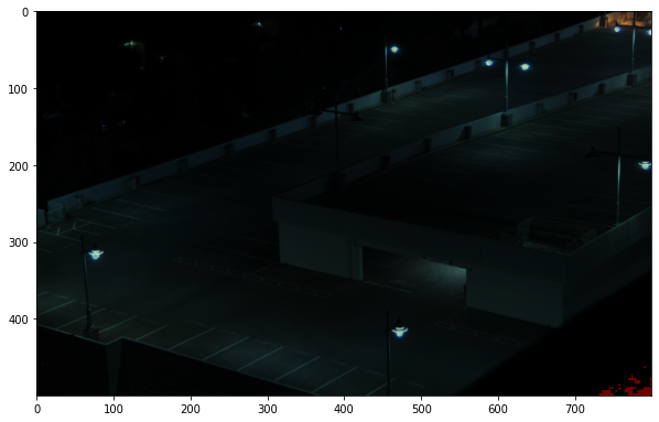
For our last project, we chose to implement "Recovering High Dynamic Range Radiance Maps from Photographs" by Debevec and Malik. The goal of this paper is to generate HDR images from a series of LDR images. Below is an example of an LDR dataset, as we can see some images suffer from overexposure while others suffer from underexposure.
|
|
|
|
|
|
|
|
|
|
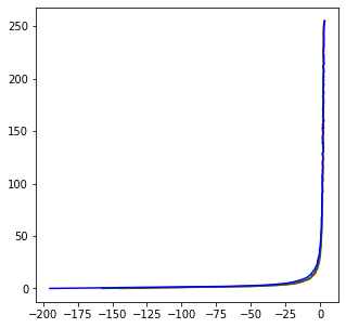
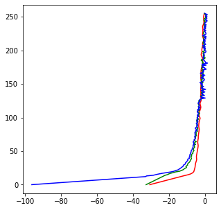
In order to achieve this goal, there are two main steps. The first involves calculating the radiance maps of an image so that we can identify which regions of the image must be bright and which must be dark and light. To do this we average the observed pixel value at each pixel for all images in the set of images. We weight observed pixel value by the reciprocal of the distance to 127.5 which we define as the center and as in the paper, we add the log of the exposure. To calculate the radiance map, we solve a least squares problem to determine which function maps our observed pixel values to the log of the exposure value. From that, we are able to calculate the function g for each color channel which will allow us to determine the exposure of the HDR image. Below is an example of the g we calculated using the garage data and the memorial data.
|
|
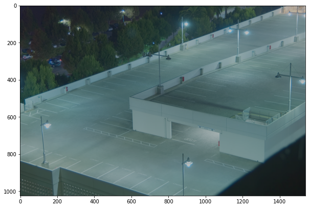
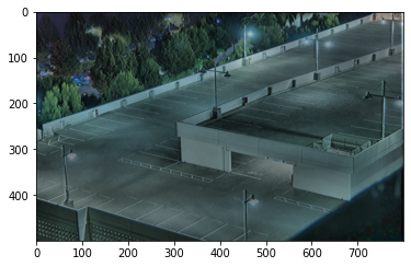
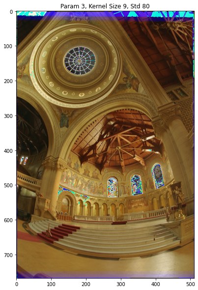
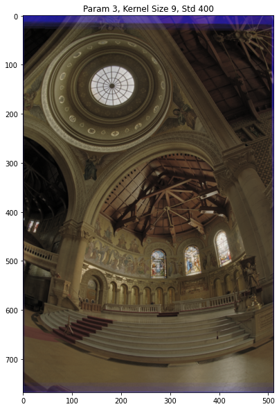
Using these, we solved for our radiance maps which we then used to construct our HDR Images. We have included outputs for both datasets below using different tone normalization schemes for each result. We used a local tone mapping algorithm as suggested in the document and have included multiple parameter results. We also used a global tone mapping algorithm from OpenCV which performed worse than the local tone mapping. We noticed that the results generated by the tone mapping algorithm from the paper appeared to be a bit washed out. As per Anonymous Atom's suggestion in Piazza, we added a custom contrast function which utilizes cv2.addWeighted to add an image to a higher-contrast version of itself. This combined with the tone mappign algorithm yielded the best results.
|
|
|
|
|
|
|