Poor Man's Augmented Reality
Gathering keypoints
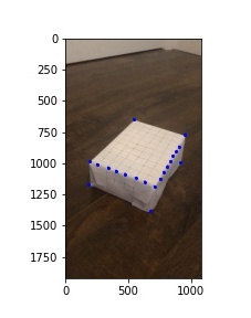
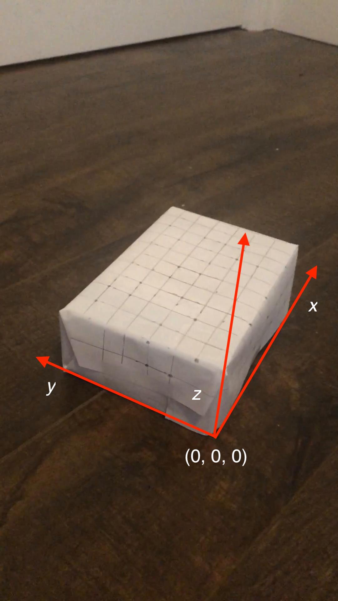
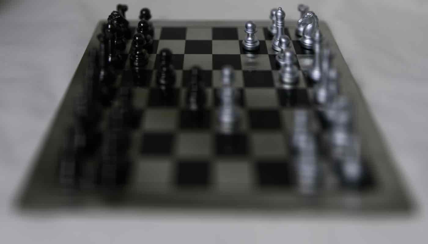
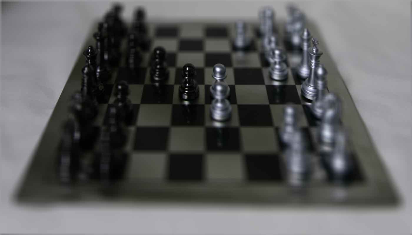
I first manually inputted coordinates in each frame using ginput. I then manually inputted the corresponding world coordinates using known measurements from the pattern on the box, with each square being 1.5cm x 1.5cm, and orienting the origin as in the image below.
Manually inputted keypoints for first frame
Orientation for world coordinates
Propogating keypoints to other frames
To propogate the keypoints to the frames, I used an off the shelf tracker approach with cv2.TrackerMedianFlow_create(). I created a tracker for each keypoint and initialized it with a bounding box of size 8x8 centered around the keypoint. From there I updated the tracker at each frame, acquiring the updated bounding box and putting the new keypoint at the center of the updated bounding box.
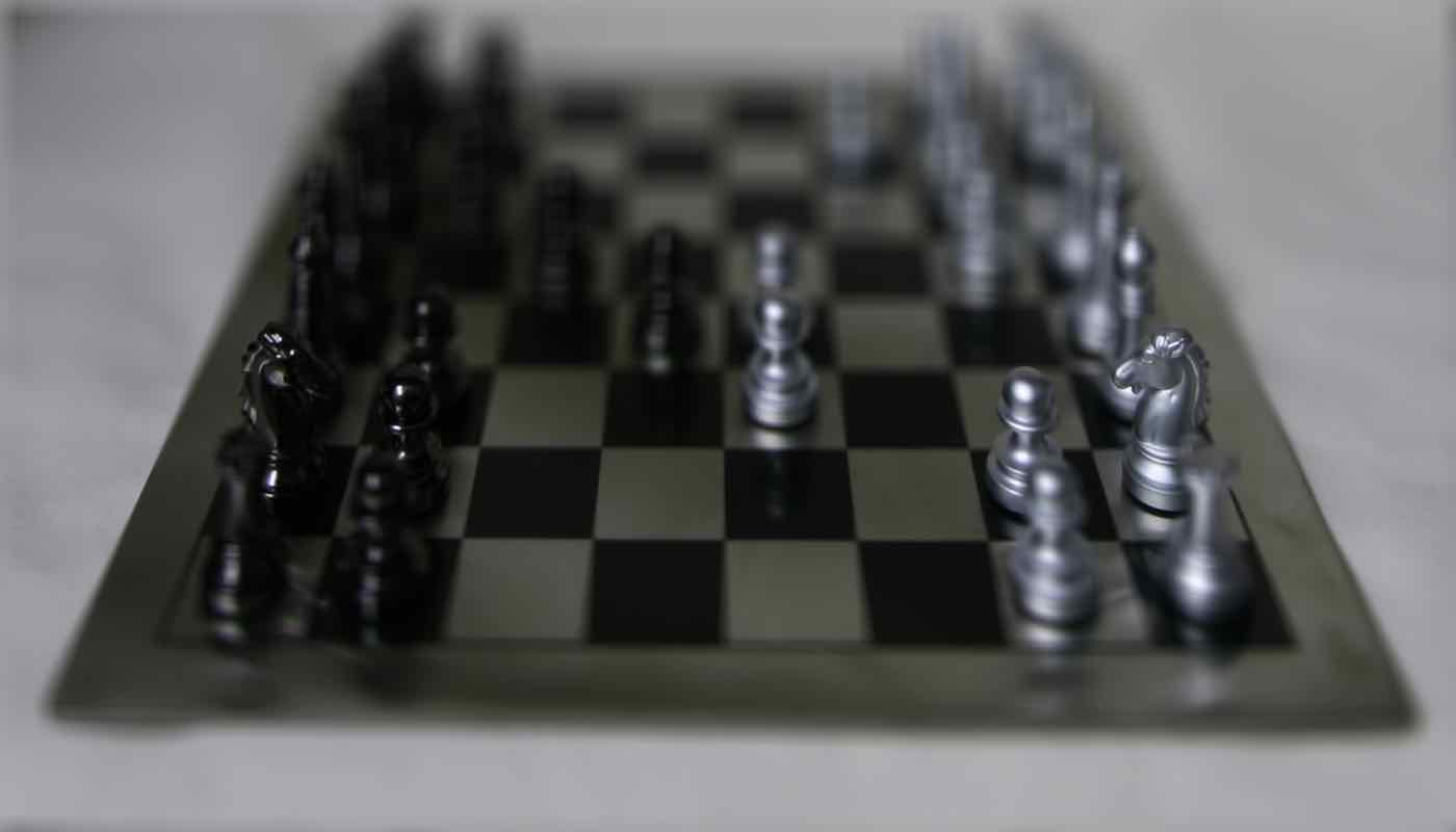
Input video
Video with keypoint tracking
Calibrating the camera
To calibrate the camera, we know that the projection matrix (composed of extrinsics and intrinsics) transform world coordinates (X, Y, Z, 1) into image coordinates (u, v, 1), as shown below.
$$
\begin{bmatrix}
su \\
sv \\
s
\end{bmatrix}
=
\begin{bmatrix}
a & b & c & d \\
e & f & g & h \\
i & j & k & 1 \\
\end{bmatrix}
\begin{bmatrix}
X \\
Y \\
Z \\
1
\end{bmatrix}
$$
Rearranging the equations given the system above yields the following:
$$ \textrm{Equation 1: }ax + by + cz + d - uix - ujy - ukz = u $$
$$ \textrm{Equation 2: }ex + fy + gz + h - vix - vky - vkz = v $$
Using the known correspondences of world coordinates and image coordinates, we can create the a system of equations using equation 1 and equation 2 on each corresponding pair, shown below.
$$
\begin{bmatrix}
X_1 & Y_1 & Z_1 & 1 & 0 & 0 & 0 & 0 & -u_1X_1 & -u_1Y_1 & -u_1Z_1 \\
0 & 0 & 0 & 0 & X_1 & Y_1 & Z_1 & 1 & -v_1X_1 & -v_1Y_1 & -v_1Z_1 \\
. \\
. \\
. \\
X_n & Y_n & Z_n & 1 & 0 & 0 & 0 & 0 & -u_nX_n & -u_nY_n & -u_nZ_n \\
0 & 0 & 0 & 0 & X_n & Y_n & Z_n & 1 & -v_nX_n & -v_nY_n & -v_nZ_n
\end{bmatrix}
\begin{bmatrix}
a \\ b \\ c \\ d \\ e \\ f \\ g \\ h \\ i \\ j \\ k
\end{bmatrix}
=
\begin{bmatrix}
u_1 \\ v_1 \\ . \\ . \\ . \\ u_n \\ v_n
\end{bmatrix}
$$
We can then solve for the system of equations to restore the unknown projection matrix.
Projecting a cube into the scene
I then projected a cube into a scene by defining object coordinates for a cube and then projecting those points using the calibration matrix for that frame. I repeated this for each frame to propogate the cube throughout the frames.
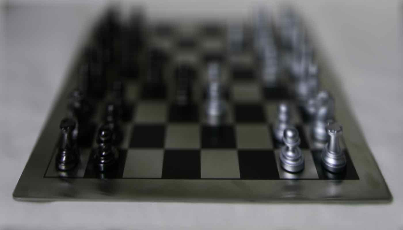
Light Field Camera
Using light field images allow us to create synthetic photographs by resorting the rays. The light field project reiterated the power of averaging that we visited in project 3 in computing the mean face of a population and using that to manipulate photos. Similarly, with light fields, averaging can produce realistic camera effects that were not in the original photo(s), so it was interesting for me to see that the idea of the power of averages can apply to other things to also create fascinating effects.
Depth Refocusing
Without shifting images, objects far away don't move as much as objects in the front and thus the images are aligned in the back and averaging all the grid images results in focus in the back. To refocus we can align the grid images according to the center of the grid.
For image at (x, y) in the grid, we apply a shift on it, which is the difference between (x, y) and the center of the grid (8, 8). The center is (8, 8) because the grid is 17 x 17. We scale the shift by some constant, and the choice of the constant's value will result in a different focus point. In the images below we see that the smaller scale factors put the focus more in the back and a larger scale factor moves the focus towards the front of the board.
scale_factor = 0
scale_factor = 1
scale_factor = 2
scale_factor = 3
Refocusing over a range of scale factors from -1 to 3.
Aperature Adjustment
For aperature adjustment I included a subset of the grid images, using fewer to get a smaller aperature. To do so I defined a radius of the aperature and included only those images that were within the neighborhood of the common point.
For example, to focus on the back of the image, I only included images in the radius x radius sized patch centered at the common point, which for the back of the image is (8, 8).

Aperature at various radii: 0, 2, 4, 6, 8
Bells and Whistles: Interactive Refocusing
To implement interactive refocusing, I applied the refocus function that I used earlier with various parameters in the range [-3, 3], with a step size of 0.5. I created a patch of size 100 x 100 centered at the pixel that should be focused (some input x, y) using the center image of the grid (unaveraged). I then computed SSD error between that patch and the same patch location sampled from the refocused images, outputting the image with the lowest SSD score as well as its corresponding scale_factor parameter.
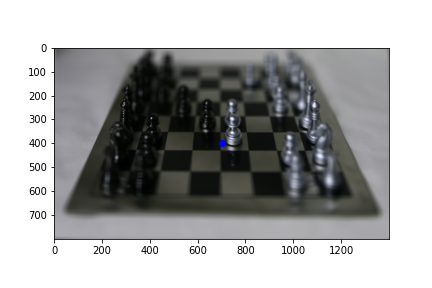
Below are some refocused images, with the selected focus point in blue. We see that for points that are equally far away in depth (bottom row) the best fit parameter is the same since the parameter implicitly represents the depth of the pixel.
scale_factor = 2.5, focus point = (220, 600)

scale_factor = 0.0, focus point = (400, 100)

scale_factor = 1.5, focus point = (700, 400)
scale_factor = 1.5, focus point = (1100, 300)
