The three projects that we elected to do were: A Neural Algorithm of Artistic Style
, Lightfield Camera: Depth Refocusing and Aperture Adjustment with Light Field Data,
and Poor Man's Augmented Reality.
Final Project: A Neural Algorithm of Artistic Style
Setting up the Model
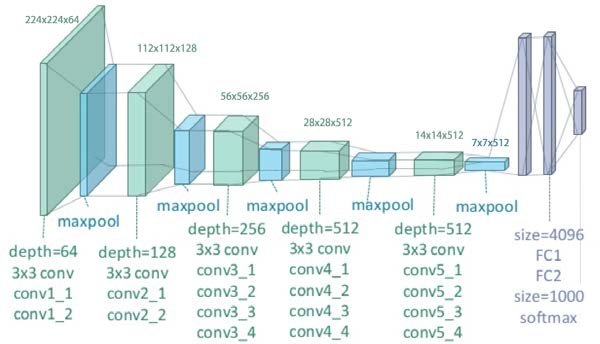
For this project, we will use a pretrained VGG-19 model, which is available from PyTorch.
Then we will proceed to only take the feature maps resulting from 5 layers.
This would be Conv1_1, Conv2_1, Conv3_1, Conv4_1, Conv5_1, which will be the first
convolution layer after a Max Pool layer.
VGG 19 Architecture
Loss Functions
This is the key functions of the paper, as these loss functions will be how
the style will be transfered.
The loss functions will be split into two: Content Loss and Style Loss.
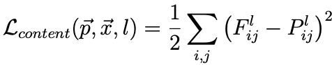
We will first discuss the content loss function, which is defined below.
Content Loss Function
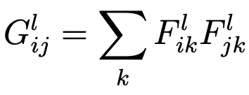
We then discuss the style loss function. First we would have to calculate the Gram Matrix.
This matrix is used to relate between different feature maps created by different filters.
Gram Matrix Equation
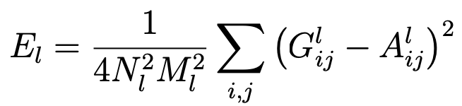
We then calculate each layer's contribution to the total loss function. G
is the Gram matrix that we just calculated. A is the Gram matrix of the original images.
We take the mean-squared distance between the two.
Gram Matrix Equation
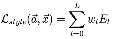
The total style loss function is calculated through the combination of the weights.
Weighted Combination Equation
Last but not least, we then combine the two loss functions together. In addition, we weight each
loss function by alpha and beta.
Loss Function Combination
Training
For the training, we can adopt a similiar process from the previous project.
However, we change the variable that the optimizer updates to our target image.
For the alpha and beta, we use the ratio that was set by the paper to be 1e-4, which
is setting alpha to 1 and beta to 1e4. I also tested different learning rates, which are shown below.
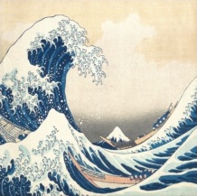
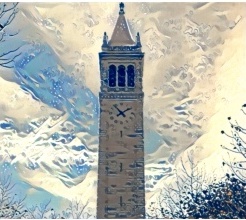
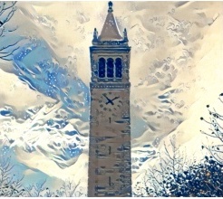
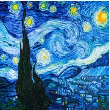
The Style Image
Learning Rate 0.03
Learning Rate 1e-4
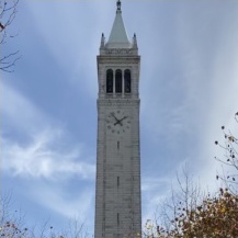
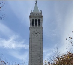
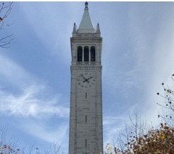
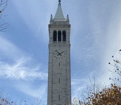
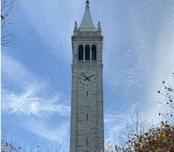
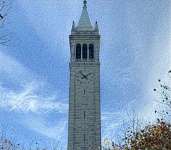
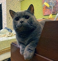
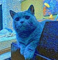
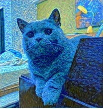
Original Images
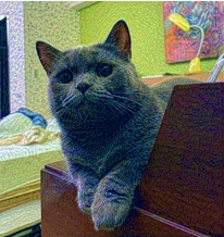
After 400 iteration
After 1200 iteration
After 2000 iteration
After 2800 iteration
After 3600 iteration
After 4400 iteration
After 5000 iteration
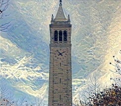
We can see that with a higher learning rate the results are better!
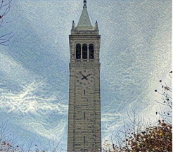
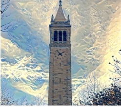
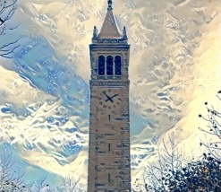
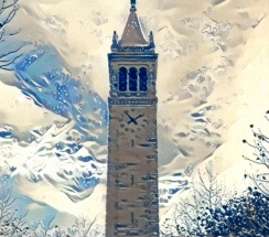
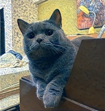
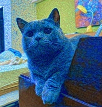
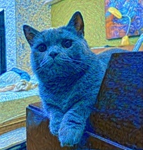
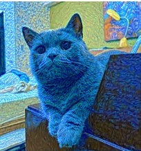
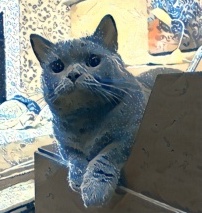
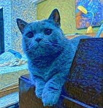
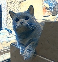
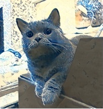
Results
The results are shown below. With the original image and the progression of the style transfer.
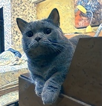
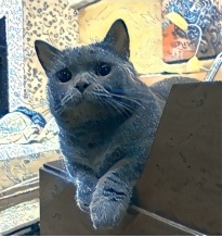
Original Images
The Style Image
After 400 iteration
After 1200 iteration
After 2000 iteration
After 2800 iteration
After 3600 iteration
After 4400 iteration
After 5000 iteration
Lightfield Camera: Depth Refocusing and Aperture Adjustment with Light Field Data
Shifting the focus
We collected a series of photos through the Stanford Light Field project.
We can first inspect the average of the images.
We can see that in the average photo, the further parts of the image is more in focus.
Average Photo
We can further change the focus of the image through re-aligning the images and applying a
constant to the shifts. The shifts are calculated through:
1. u of current image - u of middle image, v of current image - v of middle image
2. After getting those difference multiply those by alpha
3. Apply the shifts.
With a larger alpha, we will be focusing further away. On the other hand with a smaller alpha, we will be focusing
closer to the front. For the gif, I used the range (-1,1) with step size of 0.05. For the images, I showed
a couple alpha that gave us good results to show different shifts focusing at different points of the images.
Alpha = 0.1Alpha = 0.25
Alpha = 0.5Alpha = 1
The resulting gif of the shifts
Changing the Aperture
Aside from shifting the images so we can focus on different areas. We can also change the aperture size, which
in turn will change the depth of view. This can be done through checking the u, v distance of each image to the
middle image
Radius = 0Radius = 15
Radius = 30Radius = 45
The resulting gif of the different radii
Bells and Whistles
The resulting gif of the shifts on our own image of a banana:
The resulting gif of the different radii on our own image of a banana:
We don't think it worked to well because we estimated u and v (the distance to the
center of the image) instead of calculating it.
Poor Man's Augmented Reality
Setup
For the setup, we printed out a gridded paper and wrapped it around a box and took a video displayed
below
Keypoint Tracking
We selected points on the grid using plt.ginput and used a CSRT tracker to keep track of
the keypoints when we move the camera. We chose the origin of the 3D points to be the bottom left
keypoint
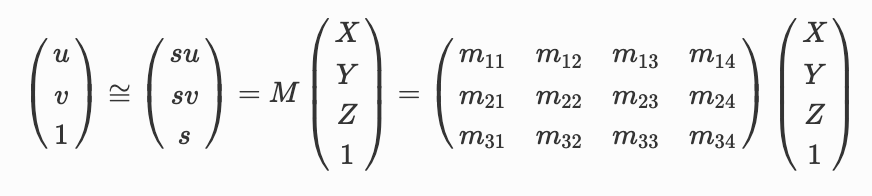
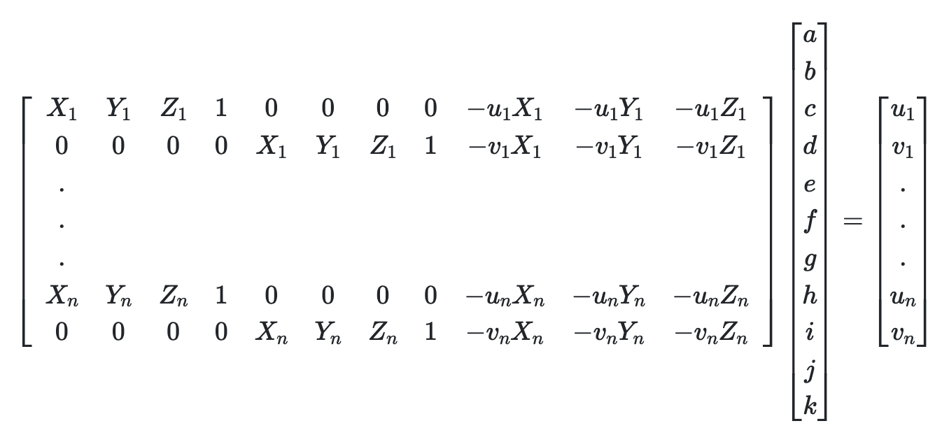
Calculating the Camera Projection Matrix
We used least squares to calculate the camera projection matrix in each frame
using the equations below.
Result
Here is the result of applying the camera projection matrix to a cube's 3D points.