Together, we completed Image Quilting, Augmented Reality, and A Neural Algorithm of Artistic Style.
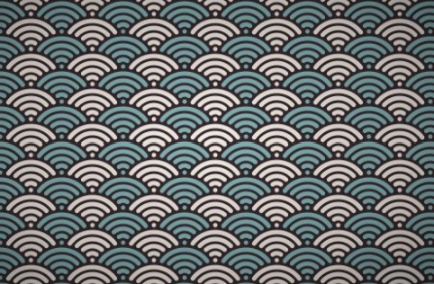
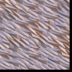
In this first project, the goal of is to implement the image quilting algorithm for texture synthesis and transfer, described in this SIGGRAPH 2001 paper by Efros and Freeman. Texture synthesis is the creation of a larger texture image from a small sample. Texture transfer is giving an object the appearance of having the same texture as a sample while preserving its basic shape
For the first part, we randomly select patches of size (patchsize, patchsize) to fill an output image of size outputsize.
For this second part, we overlap patches as we put them in the output image by the user-inputted overlap amount. We improve upon the previous method by comparing the neighboring patches to each other in hopes of making the final output more seamless. To to this, first create a list of all possible patches that can be sampled from the sample. Then, as we are building out the output image, we get the template and compute the cost of all the possible patches where they overlap with the template. Of the samples that have an error of min_cost * (1 + tol), randomly sample one to put in the respective area of the output image.
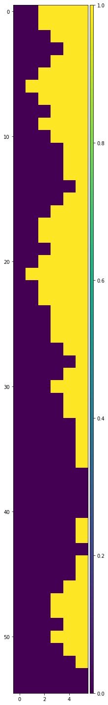
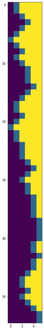
For seam finding, we improve upon just overlapping by adding another cost component. By finding the lowest cost path from left to right for horizontally overlapping images, and top to bottom for vertically overlapped images, we can creat a better seam when overlapping images.
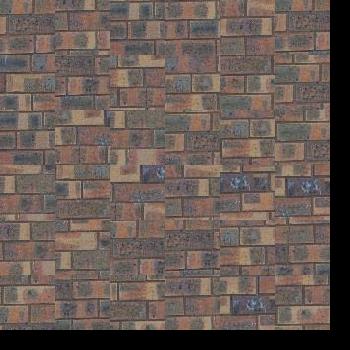
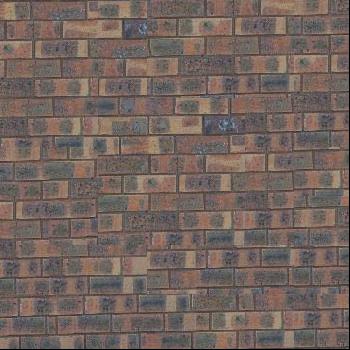
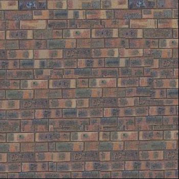
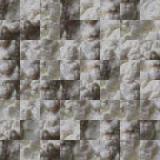
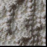
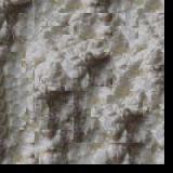
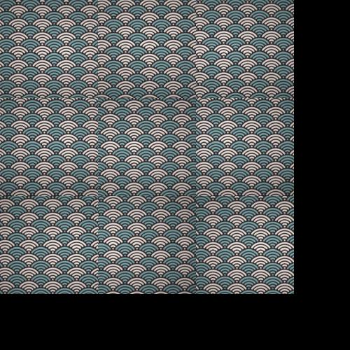
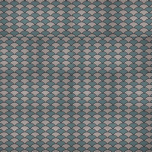
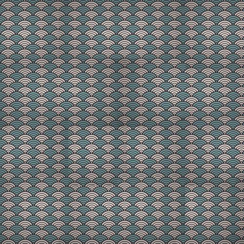
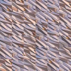
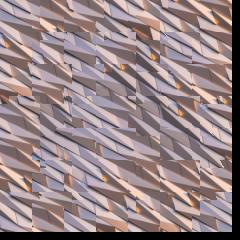
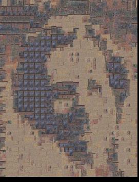
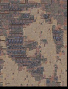
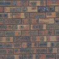
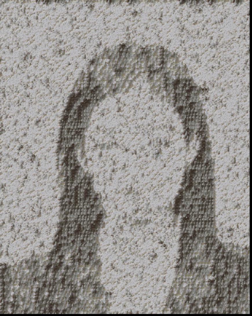
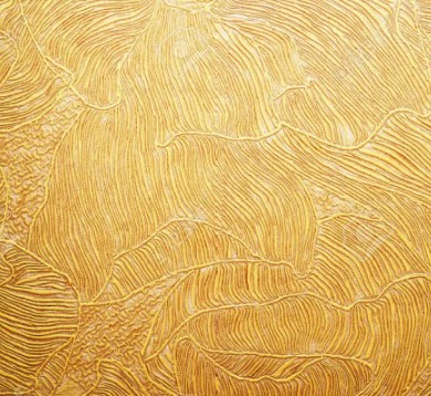
My own images are used in the following images below. The orignal images were quilted to a larger output image.

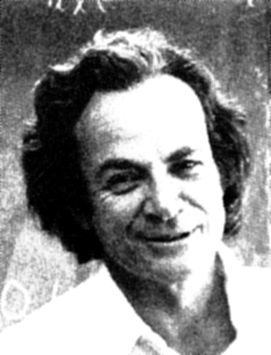
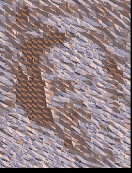
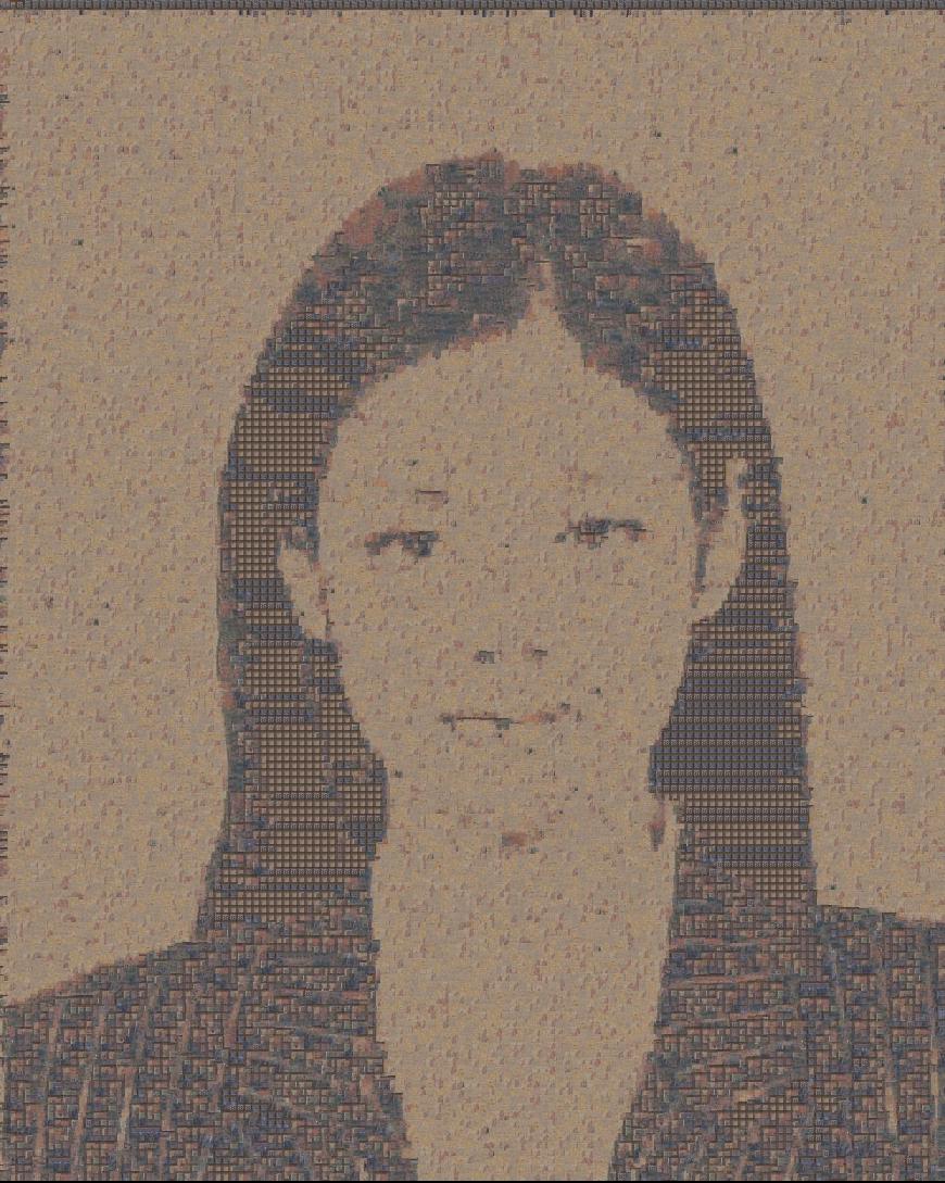
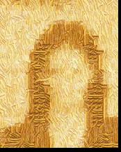
Texture transfer is building upond seam finding. The cost function we used in seam findng helped us make sure that neighboring patches are similar enough to not result in a harsh seam. For texture transfer, we add another component to the cost function. In addition to comparing patches to the ones they are overlapping, we also want to measure how similar the patch is to the target image. In order to do so, we add a SSD of the patch in black and white, and the corresponding target image patch in black and white. This is comaring the luminance in order to capture how similar the texture and the target image are. Then, the final cost value = alpha * seam_cost + (1 - alpha) * luminance_cost. We still are finding a random patch that has a cost within min_cost * ( 1 + tol) like we did in overlapping patches and seam finding.


We created our own verysion of cut.m based on the paper. It can be viewed in the jupyter notebook. To create another version of cut.m in python with dynamic programming, we first generated a cost matrix of the costs to get to each pixel, the costs being the cost of the current pixel + the cost of the path up to that pixel from the left side. Then, we backtracked from the lowest final cost to get the lowest cost path, and generated a mask from this path.
To make measuring easier, we used a Rubik's cube as the rectangular box to video. The video captured was 6 sec long with the cube in the center.
Using plt.ginput, we selected the points at all the corners on the Rubik's cube, amounting to 37 points in total. We also created a world_map that indicates the coordinate axis of the Rubik's cube. The bottome corner of the cube touching the table was (x=0, y=0, z=0). The red side is the y-axis and the white side is the x-axis.
To propagated the points, we used cv2.TrackerMedianFlow_create(). Using the coordinates we collected from the previous part, create a separate tracker for each point and pass in the bounding box to the tracker. At each frame, update the tracker and show the updated point on the image frame.
Here, we calculate the homorgraphy from 2D to 3D space following the below image:
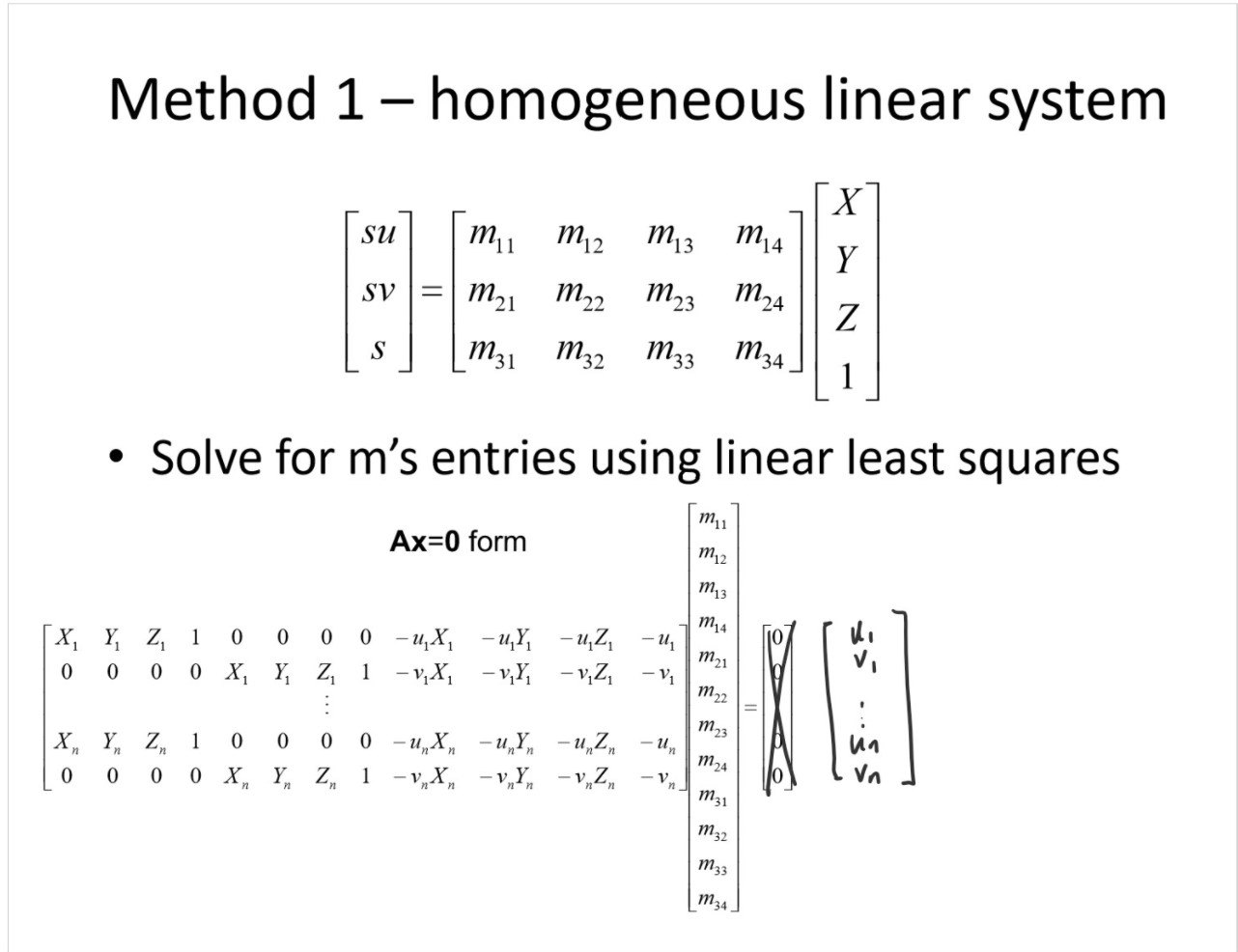
Using this, we can use the updated points at each from to calculate what the homography matrix should be to help up with projecting a cube in the next part.
For the cube, we started off with it's world coordinates and at each frame, found the homography that could transform the coordinates to the respective ones in the frame.
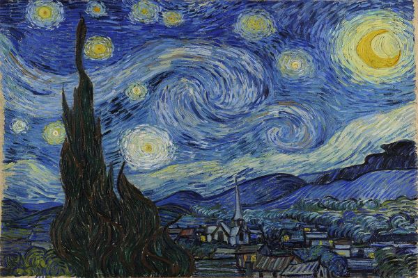
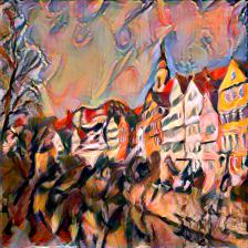
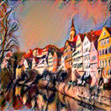
In this project, we reproduced the "A Neural Algorithm of Artistic Style" paper to the extent that the paper describes. We used vgg-19, reproduced results with the images in the paper (Composition VII and the image of Germany), and used the same losses (with constant scaling factors), ratios of weights (10e-2 to 10e-5) as well as the same layers in the vgg-19 net that were specified. Unlike the paper (because it was not specified/given), we trained each image for 500 epochs with Adam-optimizer, and the Composition VII image was slightly different (with more muted colors than what appeared to be shown on the paper) because the image of the painting we found online differed a bit. Also, image outputs were clipped.
In order to generate the features of the layers specified in the paper (conv1_1 through conv5_1, which we took to mean the first convolutional layer in each respective block of conv layers), we created a wrapper of the VGG model (as another nn.Module) that had a modified forward pass. We ran the input through the model layer by layer, saving the output of the layer if it was one of the convolutional layers of interest, and modifying the layer before passing the image through into an average pool if the layer was originally a max pool. Then, the 5 relevant features were returned from the forward pass.
For efficiency, we only get the features for the style and content images once, before entering the training loop. We do this simply by passing the style and content images into the VGG wrapper model, and saving the outputs. These are later used in different combinations to calculate losses to train our final image.
As specified in the paper, we used squared-distance or MSE loss for the content. MSE loss is also used for style, although with some pre-processing. Instead of passing in the features directly into the style loss, we pass in the gram matrices for the features, as specified in the paper. The loss for each layer was divided by N**2 *Mfor the layer, to account for the sizing of each layer contributing to larger MSE loss (we do not use M**2 because MSE loss is already divided by M). We used conv4_1 for the content loss for the CompositionVII/Germany images, and all of the layers for all of our other generated results, and varied the number of layers (1 through n) used for the style loss, as in the paper. We also had a hyperparameter for the weights of each loss.
We used the content image as the initial input image to train on. We used Adam optimizer, with the parameters as simply the image. At each step, we passed the image through our vgg-19 wrapper to get the features to calculate loss on.
| Victor | Starry night | Victor + starry night, alpha = 0.5 |
|---|---|---|
 |
 |
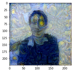 |
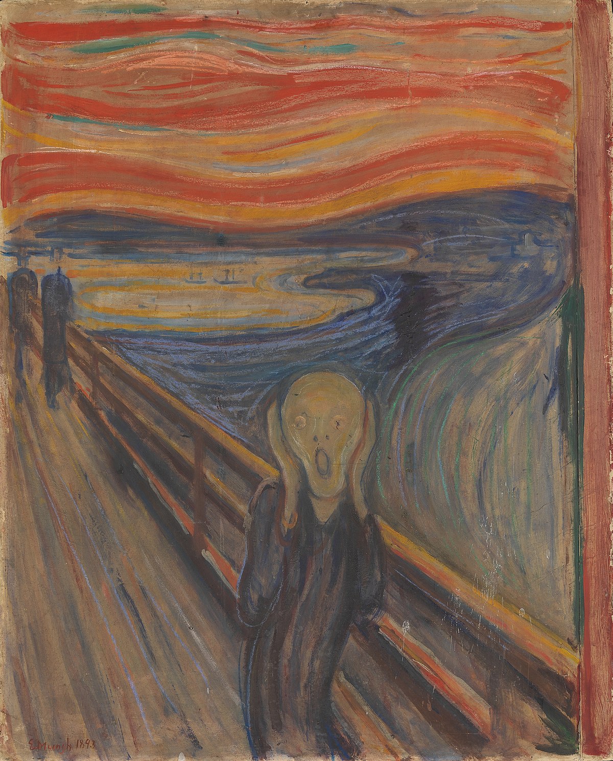
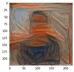
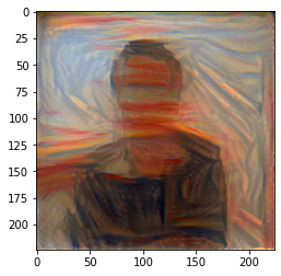
| Victor | Scream/th> | Victor + scream, alpha = 0.9 | Victor + scream, alpha = 0.5 |
|---|---|---|---|
|
 |
 |
 |
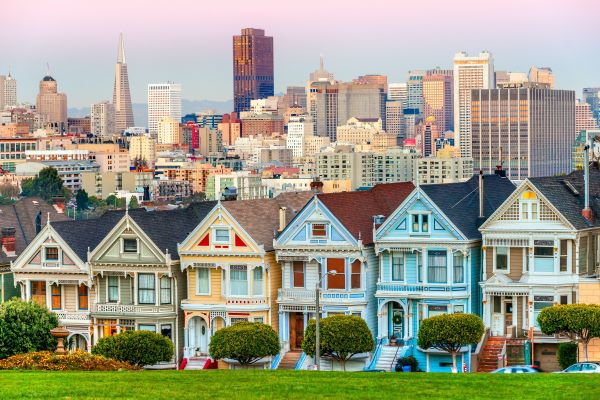
| Painted Ladies | Starry night | Painted ladies + starry night, alpha = 0.1 |
|---|---|---|
 |
|
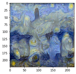 |
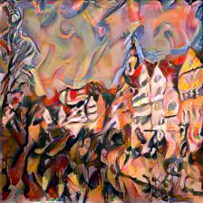
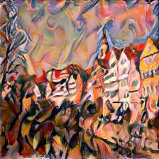
Below are some results of composition VII and Germany. We calculated alphas (defined in our code differently than in the paper) such that the ratio of style/content loss weights were the same as in the paper. Our image of Composition VII is more muted in color than the one used in the paper, and we used conv4_1 instead of conv4_2 for the content loss. These used all layers for style, and from left to right had a/B ratios of 10^-5 through 10^-2 as in the paper.
 |
 |
 |
 |