Final Project

Project 1: Lightfield Camera

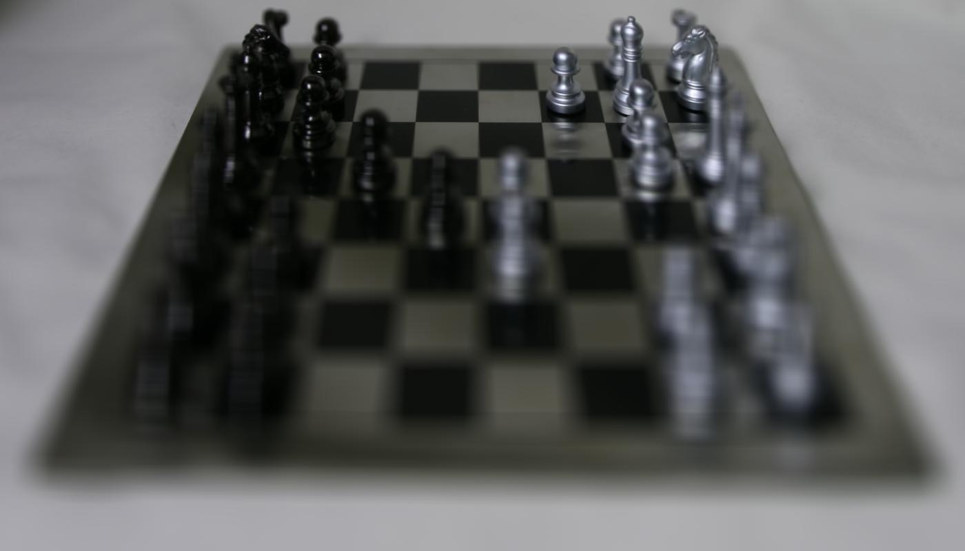
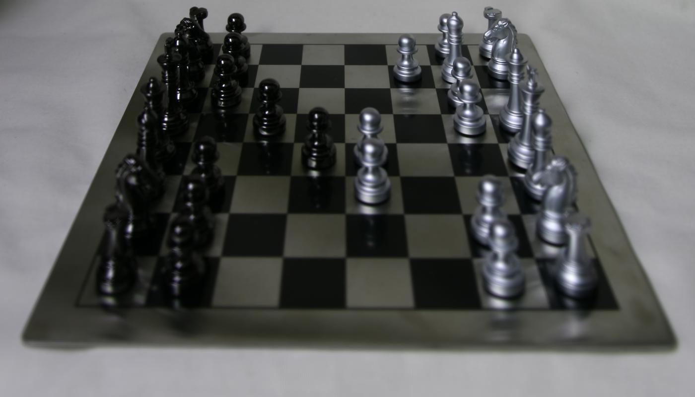
In Ng et al, a hand-held lightfield camera is used to capture many images perpendicular to the optical axis, allowing complex effects such as post-hoc depth-based refocusing and aperture adjustment with simple averaging and shifting tricks. In this project, we use lightfield data from the Stanford Lightfield Archive to demonstrate these effects.

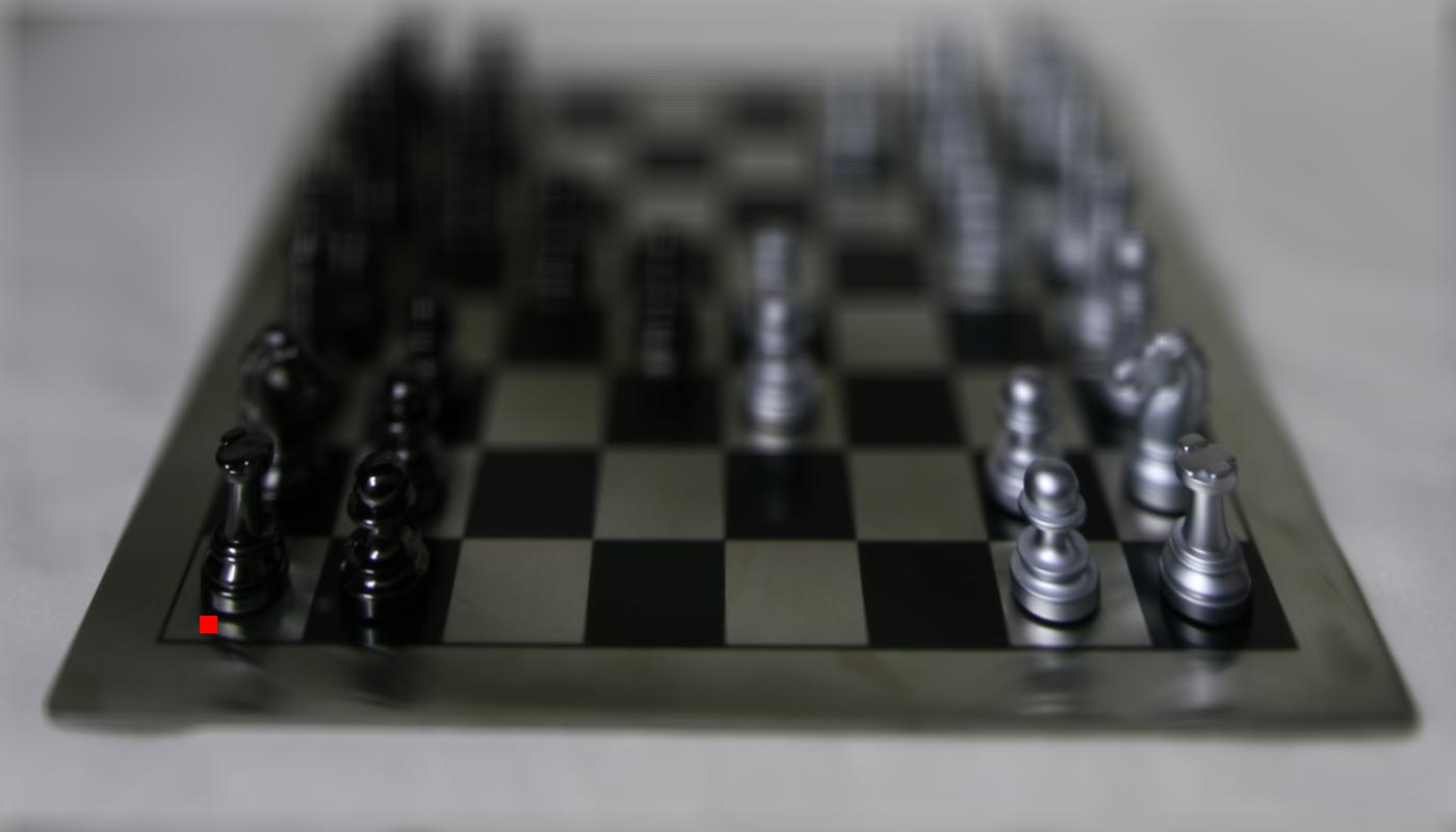
Depth Refocusing

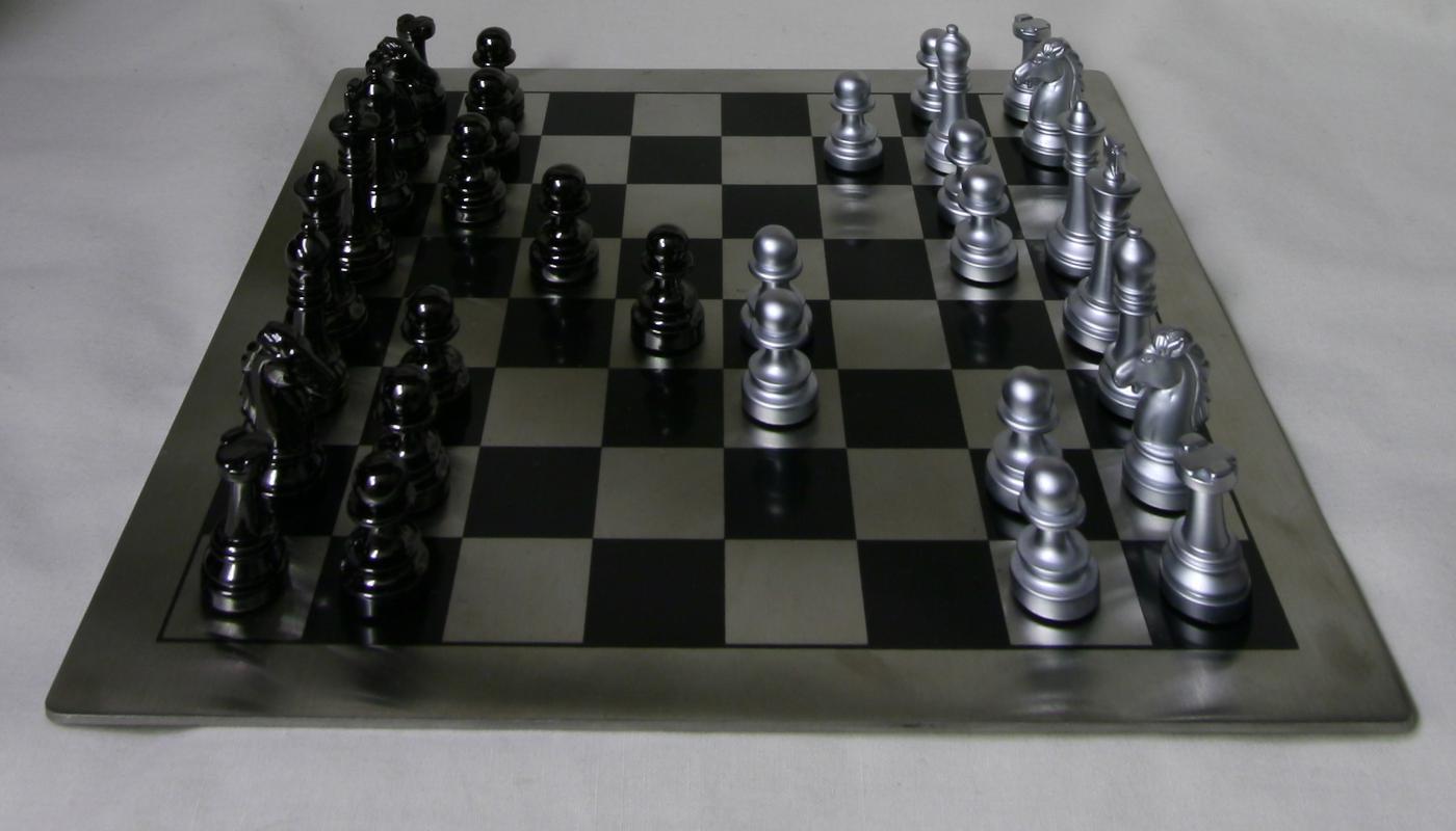
A naive averaging of all the sub-aperture frames (no shifting) yields an image where the far away objects are in focus and the nearby objects are blurry. By shifting the images proportional to their distance from the center (scaled by a depth parameter alpha which is user-controlled), we can appropriately shift the images such that objects at varying depths are in focus. We perform this by shifting an sub-aperture image by (alpha * (x - cx), alpha * (y - cy)) where (x, y) is the sub-aperture image's camera position and (cx, cy) is the camera position of the center image at grid position (8, 8). Changing alpha (as shown below) results in refocusing at various depths.

Aperture Adjustment

A single image will have the entire frame in focus and a small aperture. We can simulate a larger aperture by averaging more images within a specified radius of the initial image because this will simulate more light coming in from different directions. We chooose our single image (radius = 0) to be the center image at grid position (8, 8) and as we increase the radius we average in images with grid positions which are within the specified radius of (8, 8). Setting the radius to be arbitrarily large will cause many images to be averaged together, simulating a larger aperture and causing more elements to blur.

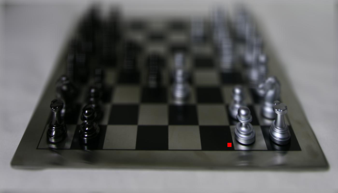
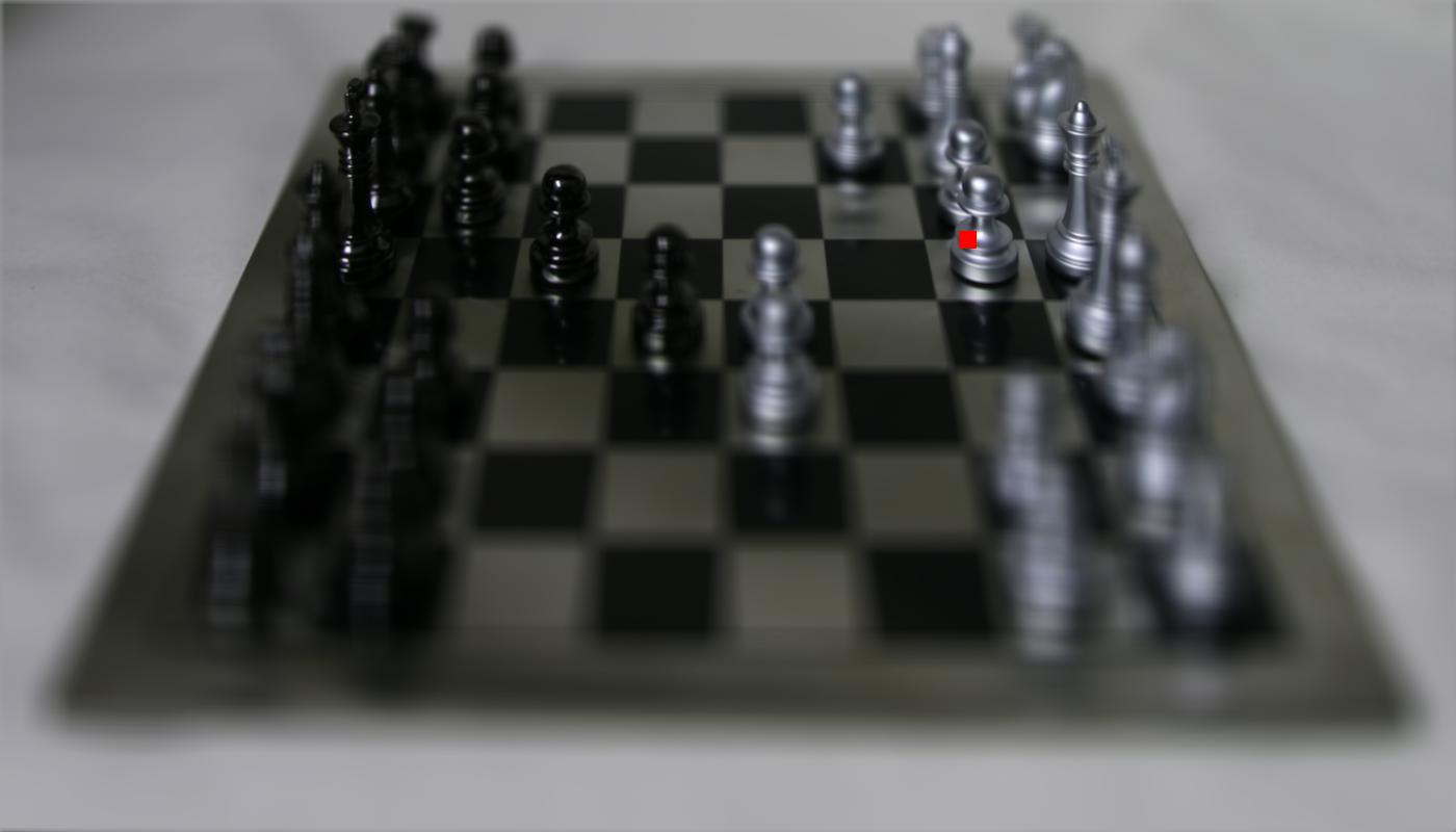
B&W: Interactive Refocusing

We can interactively refocus lightfield data by computing the depth parameter (alpha) from a user-provided (x, y) coordinate. We do this by comparing a 100x100 patch around the point of interest in the (8, 8) sub-aperture image and another non-center image. We perform shifts on the non-center image using the same shifting technique (in terms of an alpha parameter) used for depth-refocusing. We search over 201 alpha values uniformly spaced on [-1, 1] and greedily select the alpha value that minimizes the sum of squared distances (SSD) between the two image patches. Once we have this optimal alpha parameter, we can perform standard depth refocusing with this alpha parameter to focus the scene on the user-provided (x, y) point.

Summary

Project 2: Neural Style Transfer

Method

We re-implemented the method described in Gatys et al with some minor modifications. The goal is to transfer the texture from a painting ("style image") onto a photograph ("content image") while still preserving semantics in the final generated image. This is done by jointly optimizing a content loss and a style loss with gradient descent for an input image.

We start with a pre-trained VGG19 architecture, and replace the max pooling operations with average pooling operations based on the suggestion in Gatys et al. We found that the results were significantly improved with average pooling. We also remove the fully-connected layers (the classification head) from the model. The architecture of our modified VGG19 is below:

Sequential(
    (0): Conv2d(3, 64, kernel_size=(3, 3), stride=(1, 1), padding=(1, 1))
    (1): ReLU(inplace=True)
    (2): Conv2d(64, 64, kernel_size=(3, 3), stride=(1, 1), padding=(1, 1))
    (3): ReLU(inplace=True)
    (4): AvgPool2d(kernel_size=2, stride=2, padding=0)
    (5): Conv2d(64, 128, kernel_size=(3, 3), stride=(1, 1), padding=(1, 1))
    (6): ReLU(inplace=True)
    (7): Conv2d(128, 128, kernel_size=(3, 3), stride=(1, 1), padding=(1, 1))
    (8): ReLU(inplace=True)
    (9): AvgPool2d(kernel_size=2, stride=2, padding=0)
    (10): Conv2d(128, 256, kernel_size=(3, 3), stride=(1, 1), padding=(1, 1))
    (11): ReLU(inplace=True)
    (12): Conv2d(256, 256, kernel_size=(3, 3), stride=(1, 1), padding=(1, 1))
    (13): ReLU(inplace=True)
    (14): Conv2d(256, 256, kernel_size=(3, 3), stride=(1, 1), padding=(1, 1))
    (15): ReLU(inplace=True)
    (16): Conv2d(256, 256, kernel_size=(3, 3), stride=(1, 1), padding=(1, 1))
    (17): ReLU(inplace=True)
    (18): AvgPool2d(kernel_size=2, stride=2, padding=0)
    (19): Conv2d(256, 512, kernel_size=(3, 3), stride=(1, 1), padding=(1, 1))
    (20): ReLU(inplace=True)
    (21): Conv2d(512, 512, kernel_size=(3, 3), stride=(1, 1), padding=(1, 1))
    (22): ReLU(inplace=True)
    (23): Conv2d(512, 512, kernel_size=(3, 3), stride=(1, 1), padding=(1, 1))
    (24): ReLU(inplace=True)
    (25): Conv2d(512, 512, kernel_size=(3, 3), stride=(1, 1), padding=(1, 1))
    (26): ReLU(inplace=True)
    (27): AvgPool2d(kernel_size=2, stride=2, padding=0)
    (28): Conv2d(512, 512, kernel_size=(3, 3), stride=(1, 1), padding=(1, 1))
    (29): ReLU(inplace=True)
    (30): Conv2d(512, 512, kernel_size=(3, 3), stride=(1, 1), padding=(1, 1))
    (31): ReLU(inplace=True)
    (32): Conv2d(512, 512, kernel_size=(3, 3), stride=(1, 1), padding=(1, 1))
    (33): ReLU(inplace=True)
    (34): Conv2d(512, 512, kernel_size=(3, 3), stride=(1, 1), padding=(1, 1))
    (35): ReLU(inplace=True)
    (36): AvgPool2d(kernel_size=2, stride=2, padding=0)
)
        

To create the style loss we forward the model with the style image and keep the layer activations for conv1_1 (index 0), conv2_1 (index 5), conv3_1 (index 10), conv4_1 (index 19), and conv5_1 (inidex 28). We then get the layer activations for the same layers with a given input image. We compute the Gram matrix (computed as a reshaped version of the activation such that it is a 2D matrix A and then the Gram matrix is A @ A.T) for each layer activation and add compute the MSE between the Gram matrix of each layer activation for the style and input images. As per the description in the paper, we normalize each Gram matrix by the number of elements in the activation tensor. The sum of these per-layer MSE losses is equal to the total style loss.

The content loss is computed by taking the layer activation for conv4_1 of the content image and the input image and taking the MSE between the two activation tensors.

To produce the style transfer result, we start with a clone of the content image as our starting input image. We then use LBFGS to optimize the total loss (the weighted sum of the content loss and the style loss) for 100 gradient steps and return the result. We weight style loss by 10^6 and content loss by 1.

Results

Initialization

We experimented with initializing the input from the content image and from a random uniform distribution. While the random initialization moves somewhat towards the correct shape and texture, the results initialized from the content image are far more effective.

Project 3: Gradient Domain Fusion

Overview

In this project, we explore a different method for creating composite images by blending two images together. This approach is gradient domain processing, which focuses on preserving the gradient of the image so the resulting image maintains the object structure, but not necessarily the color intensity. To do this, we implement Poisson blending, discussed in the Perez et al. 2003 paper.

Part 1: Toy Problem

Before directly implementing Poisson Blending, we started with a simpler "Toy" problem. This example will highlight that we can use the gradients of an image as well as a single pixel intensity to get the original image. To do so, we will run least squares to minimize the following objectives:

1. The difference in x-gradients of v and s:

   ( v(x+1,y)-v(x,y) - (s(x+1,y)-s(x,y)) )^2

2. The difference in y-gradients of v and s:

   ( v(x,y+1)-v(x,y) - (s(x,y+1)-s(x,y)) )^2

3. The difference in color of the top-left pixels of v and s:

   (v(1,1)-s(1,1))^

To implement these objectives, we construct A and b to solve Av = b via least squares. To do this, we create A as a sparse matrix of size (2 * H * W + 1) x (H * W), since we will have H * W constraints for the x-gradients, and the same number for the y-gradients. The "+1" is for the final top-left pixel constraint.

For the x-gradients, we set up the first H * W rows of A to be the identity matrix added to the negation of the identity matrix rolled on the row-axis by one entry. This essentiall creates the identity with the negation of the identity rolled to the right once. We set the last row of A to not have the negation, to ignore the gradient between the bottom left and top right pixel. For the y-gradients, we do the same operation but instead of shifting by one, we shift by W, which correlates to shifting a full row of pixels, hence one pixel down vertically for those gradients. The last row of A is set to be 1 at the first pixel, since the last entry in b will be the pixel value for the original image, which we want to be the same.

Since Av creates a vector calculates the gradients of v and we are computing the gradients of s to get b, we get b as b = As. Now, with A and b we solve for v using sparse least squares.

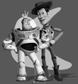
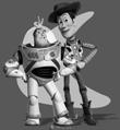
With this processing, we get the following output for the toy images.

The two images are basically identical. There seems to be some aliasing around the characters in the image, but it is clear the gradients were preserved and could generate the image we started out with.

Part 2: Poisson Blending

Moving on from the Toy Problem, we implement Poisson Blending using similar logic as before. For Poisson Blending, we need to solve the following problem:

To solve this problem, we first align the images. To do so, we use plt's ginput to get key points on both images. Then, we use the align image code from Project 2 to align the images. After the images are aligned, we use ginput again to get the key points that will outline the mask for blending.

With the mask points, we use scipy's polygon method to get the pixel locations inside the mask. Then, we move on to creating A and b as we did in the Toy problem. In this case, since we check all the neighbors, not just the x and y gradients, we have 4 constraints per pixel, requiring A to be of size (4 * n + 1) x (H * W), where n is the number of pixels in the mask. Using parallelized code, we create n x H * W matrices to represent each neighbor constraint for all the pixels in the mask, where for horizontal constraints we have 1 for each mask pixel and -1 for the horizontal neighbor, and for vertical constraints the -1 is for the pixel above or below. We repeat the last constraint from the Toy problem, constraining that the top-left pixel matches that of the original image.

For each constraint, we also make them so the neighbors in the mask result in the constraint min ((vi - vj) - (si - sj))^2. For the neighbors in the mask, we create the constraint min ((vi - tj) - (si - sj))^2. Alongside the creation of A, we fill in the b vector to match these equation constraints.

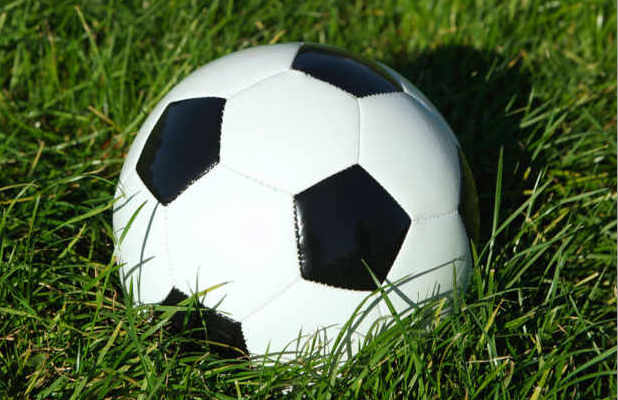
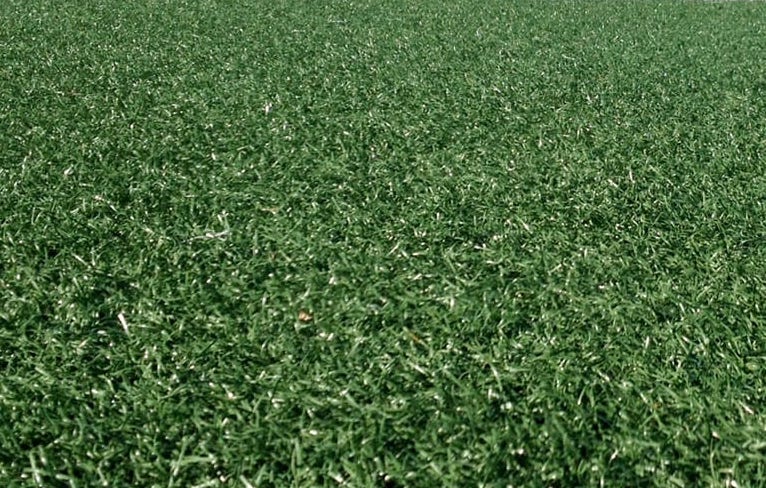
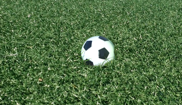
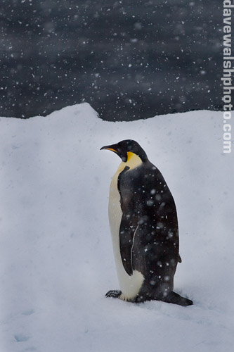
Finally, we use sparse least squares again to get the output v. We then take v, which is the pixel values in the mask, and insert those pixels into their corresponding locations in the target/background image. This results in the images below:

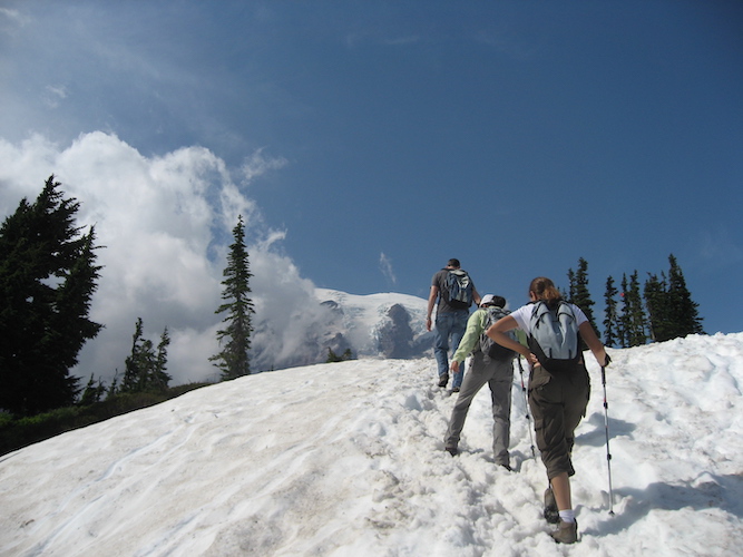
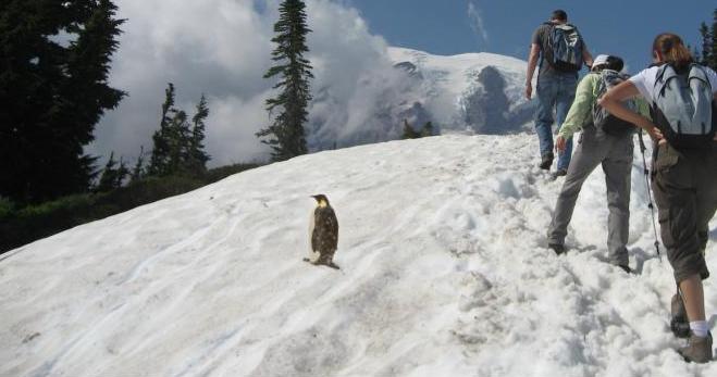
The above images represent strong blending results, where the combination of images results in no discernable unusual boundaries around the blending mask. For the soccer image, we so see some blurring around the ball, likely due to the original ball image's grass being much larger and less dense than the grass on the original pitch image, causing varying frequencies that are blurred together, but it is still a strong blend. The penguin and snow images blend very well together, evidently due to the fact that both orignal images have the similar snow background.

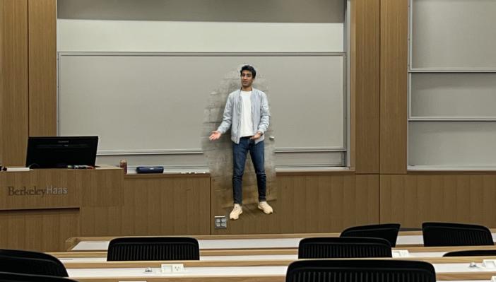
We do have the following failure case, however:

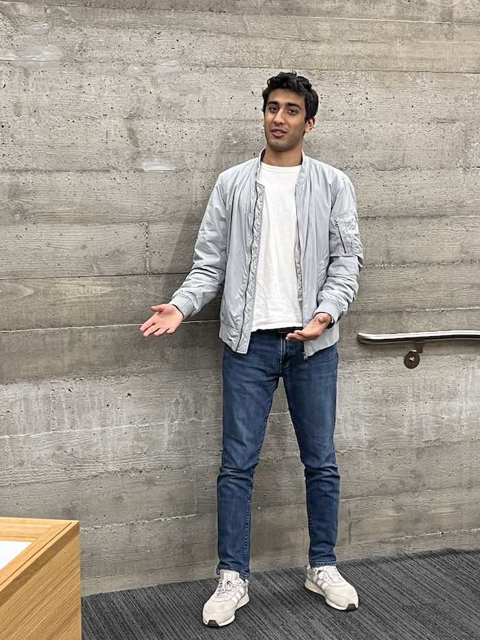
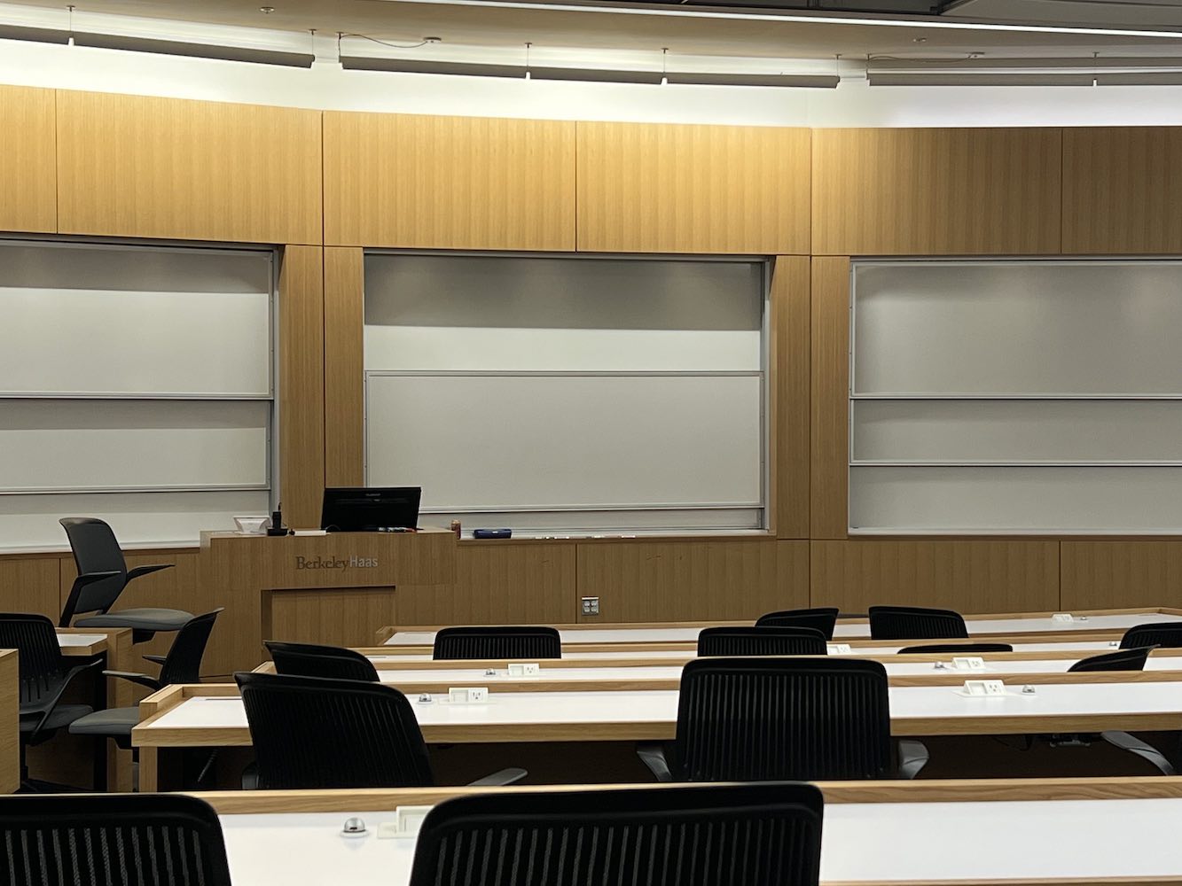
As seen above, the backgrounds of the two original images do not merge well at all. First, the grey, rugged texture in the image of Adnaan standing does not blend whatsoever with the smoother, beige and white background of the lecture hall podium. As a result, we see a blurring of the grey, white, and beige, as well as the texture in the grey concrete background behind Adnaan carrying over into the blended image, looking quite out of place.

What We Learned

This project taught us the power of gradients in mantaining the overal structure of images to blend smoothly. Furthermore, working with such large matrices, we learned how sparse matrices are very useful for efficient computation. Implementing image-wide gradients efficiently using the sparse matrices, and learning about the strengths and flaws of gradient blending were really fascinating, and expand on our original understanding of gradients from Project 2.