The goal of this project is to extract style and content from an image then transfer them to create cool hybrids.
The approach is to extract these features from Convolutional layers, using specific style and content losses to train an image to convergence.
The final output image should have a fluent mixture of both style and content elements, determined through weights.
The style of an image can be represented as a linear combination of certain convolutional layers, while the content of an image can be represented as the output of a singular convolutional layer.
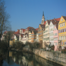
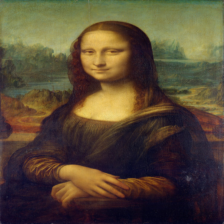
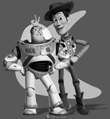
Here is the sample content image used in the paper for reference:
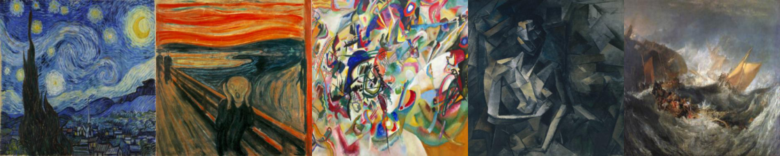
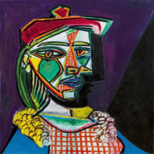
Here are the sample style images used in the paper for reference:
The Neural Network used is a pretrained VGG-19 model, where the MaxPooling Layers are replaced with AvgPooling Layers.
As per VGG standard, all style, content, and output images have shape (3, 224, 224).
As per VGG standard, all inputs must be normalized to the following means & stds across the 3 channels: [0.485, 0.456, 0.406], [0.229, 0.224, 0.225]
Since we are training an image, I added a NormLayer as the input layer before the VGG network.
Here is the full architecture of the VGG network:

In order to get our Convolutional layer outputs, I implemented hook functions as they are non-invasive.
The relevant Conv Layers are within the VGG: [0, 5, 10, 19, 28]. Note that the VGG network is truncated down to Layer 29, the ReLU layer after the last Conv Layer.
The Style Loss uses MSE Loss over Gram Matrix representations of the style image and output image divided by 4*N^2M^2, where N is the number of filters and M is height*width of the image.
The Content Loss just uses MSE Loss of the content image and output image.
The Adam Optimizer was used to train the image.
Since we want to train our image, not our network, we set the network to evaluation mode while requiring gradient for the image.
To obtain the target features for both style and content, we run both images on the network, using hooks to obtain each intermediate representation.
In order to transfer style on to an image, our input image into the network is a clone of the content image. The image is then trained to minimize both style and content loss.
The hyperparameters for the algorithm are:
# of Training Iterations
beta - overall style weight
alpha - overall content weight
per layer weights for content and style (sums to 1)
learning rate of optimizer
We decided on 1200 training iterations and 0.2 learning rate before performing hp search.
Here are the results of hyperparameter search on alpha/beta ratio and per layer weights.
Traversing down each row is an increasing subset of style layer weights ([1,0,0,0,0], [0.5,0.5,0,0,0], ... [0.2,0.2,0.2,0.2])
Traversing left to right, each column is a decreasing alpha/beta ratio (1e-2, 1e-4, 1e-6, 1e-8, 1e-10)
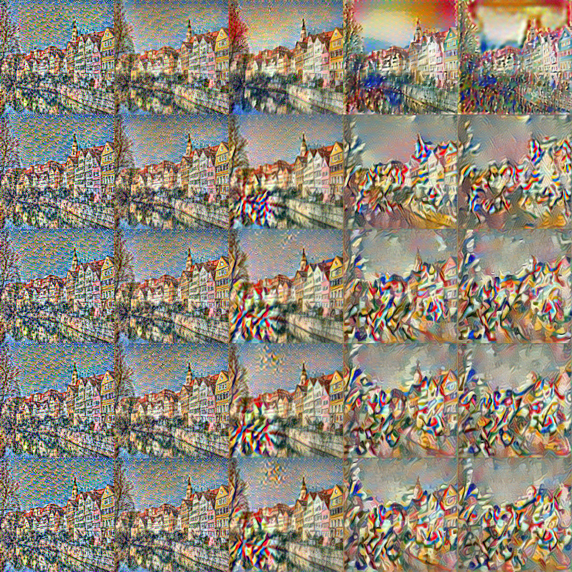
After careful scrutiny, the final alpha/beta ratio used was 1e-8 and style layer weights [0.2, 0.2, 0.2, 0.2, 0.2].
To perform style reconstruction, instead of using a copy of the content image, we use a white noise image.
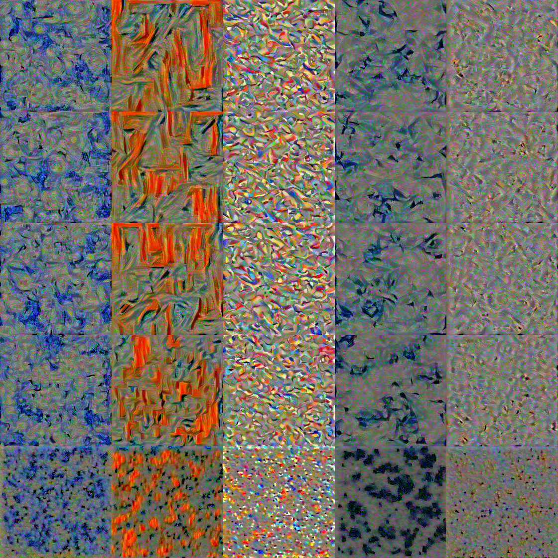
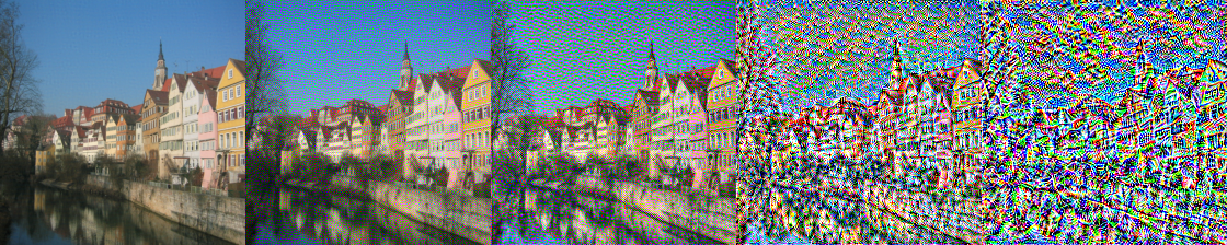
Here are the results of Style Reconstruction for all sample images compared to the raw images for reference.
Traversing down are increasing subset of style layer weights ([1,0,0,0,0], [0.5,0.5,0,0,0], ... [0.2,0.2,0.2,0.2])
To perform content reconstruction, instead of using a copy of the content image, we use a white noise image.
Here are the results of Content Reconstruction for tubingen compared to the raw image for reference.
Traversing down are one-off subsets of content layer weights ([1,0,0,0,0], [0,1,0,0,0], ... [0,0,0,0,1])
After careful examination, the [0,0,0,1,0] content layer weights was chosen for the final model.
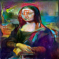
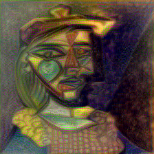
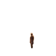
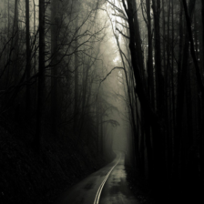
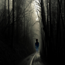
Here are the final style transfer results for all sample images listed in the paper with the raw content and style images for reference:
Content:
Style:
Transfer:
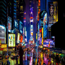
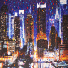
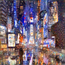
Here are some of my own Style Transfers:
Content, Style, Transfer:


This webpage contains the following two final projects: A Neural Algorithm for Artistic Style and Gradient Domain Fusion
All output images have width=224, height=224
Given our source image, s, and its dimensions (w, h), let v be a wxh array where v[y, x] maps to the flattened index. Let A be a (2*w*h, w*h) zero array and b be a 1D zero array with length 2*w*h. Following the implementation details, I iterate through each pixel for both x (Objective 1) and y gradients (Objective 2).
After populating A & b, I set A[0,0] = 1 and b[0] = s[0, 0] to satisfy Objective 3. We solve for the new image using sparse least squares from scipy.
Here are the replicated vs. original toy problem images:

Since we now have a mask area, and we are blending our source image into a different target image, the implementation is quite different.
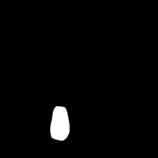
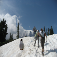
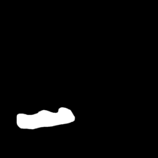
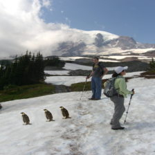
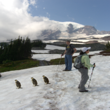
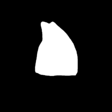
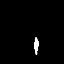
First, I made sure the source image and target image were the same size and created a mask for where the source image would be in the target.
I did this manually using a photo editor, allowing the source image to have a 4th transparency dimension with [0, 1] unique values, which was used for the mask.
With the mask coordinates, A is a (len(mask coordinates), h*w) zero array and b is a 1D len(mask coordinates) zero array. v is initialized the same way as Part 1.
Iterating through the mask coordinates, we let A[e, v[y, x]] = 4, since we are using all 4 cardinal directions. For each direction from the given pixel, we check if the neighbor is within the mask.
If it is, then we set A[e, v[neighbor_y, neighbor_x]] = -1 and subtract b[e] by (s[neighbor_y, neighbor_x] - s[y, x]). If it isn't, then we just add b[e] by t[neighbor_y, neighbor_x].
We then solve for Av = b, where v is the new output image. Note that we must solve Av=b for each color channel in the image, then stack them to get the final output image.
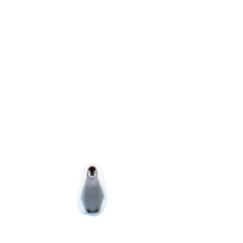
The implementation of Mixture Gradients is similar to Poisson Blending. The only change is when a neighboring pixel is within the mask, we check both the source image gradient and target image gradient, taking the one with the higher magnitude.
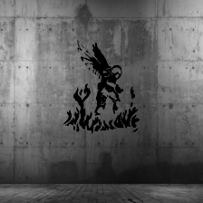
Here is a step by step process of the final results (mask, source, target, poisson blend, mixture gradient blend):
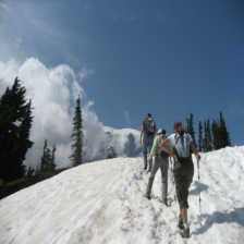

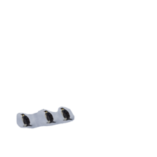
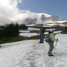
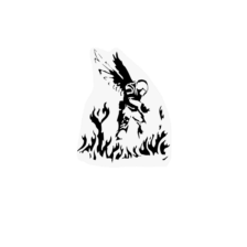
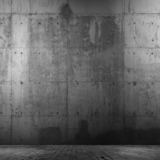
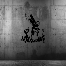

For poisson blend results, the graffiti looks unrealistic as it does not conform to the background. This is an issue where the target image background holds large gradients (not uniform).
For mixture gradient blend results, notice that the penguin chick looks translucent due to the lack of gradient in the belly. The graffiti looks more realistic as the background matches more closely.