Part 1: Loading Images
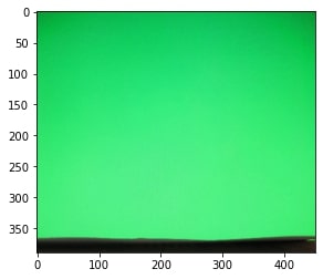
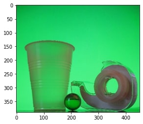
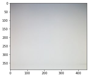
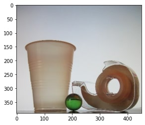
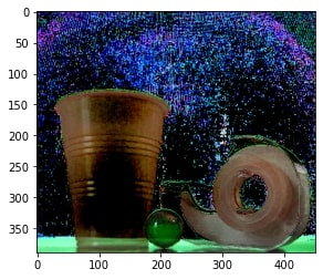
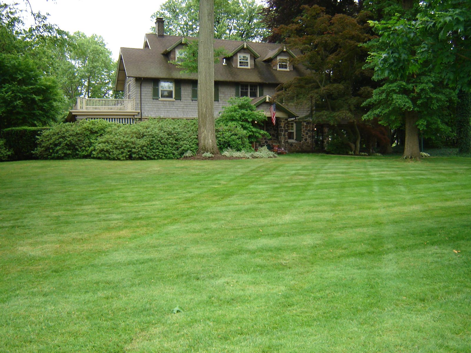
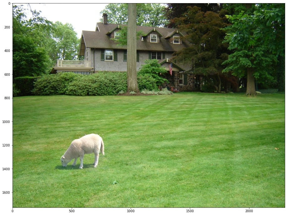
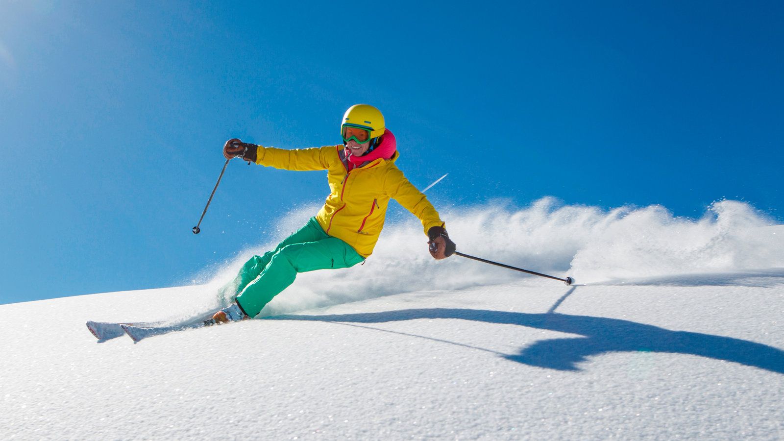
We load four images first: two images of the backgrounds and two images of the object against the backgrounds.
Some images are taken from http://cs.brown.edu/courses/csci1290/2011/results/final/aabouche/
We load four images first: two images of the backgrounds and two images of the object against the backgrounds.
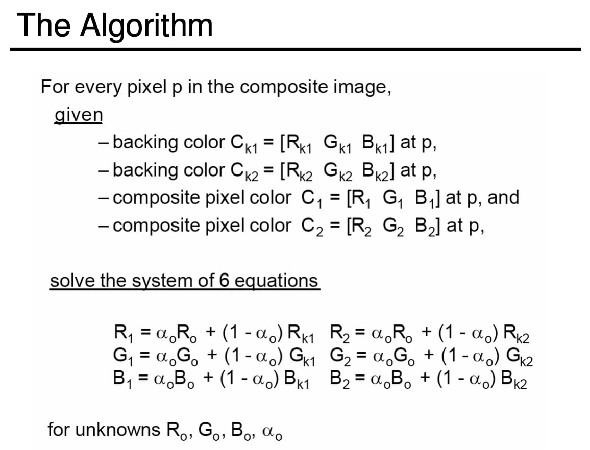
For each pixel in the image, we solved the following system of linear equations using least squares as covered in the lecture slides.
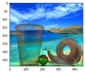
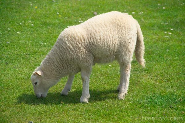
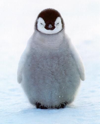
Here are the images of the object and the alpha matte.
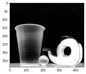
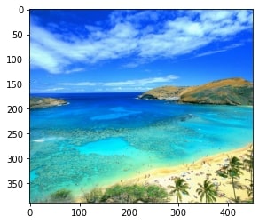
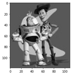
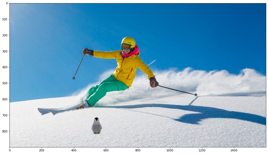
We use the alpha matte to composite the object and a new background together. Since the new background is just a generic background, no homography is needed.
We set up a system of linear equations to solve in order to reconstruct the input image, and there are three types of equations: (1) Derivatives with respect to x match (2) Derivatives with respect to y match (3) The top left conner pixels match.
We show the original image on the left, and the reconstructed image on the right. They look identical.

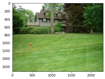
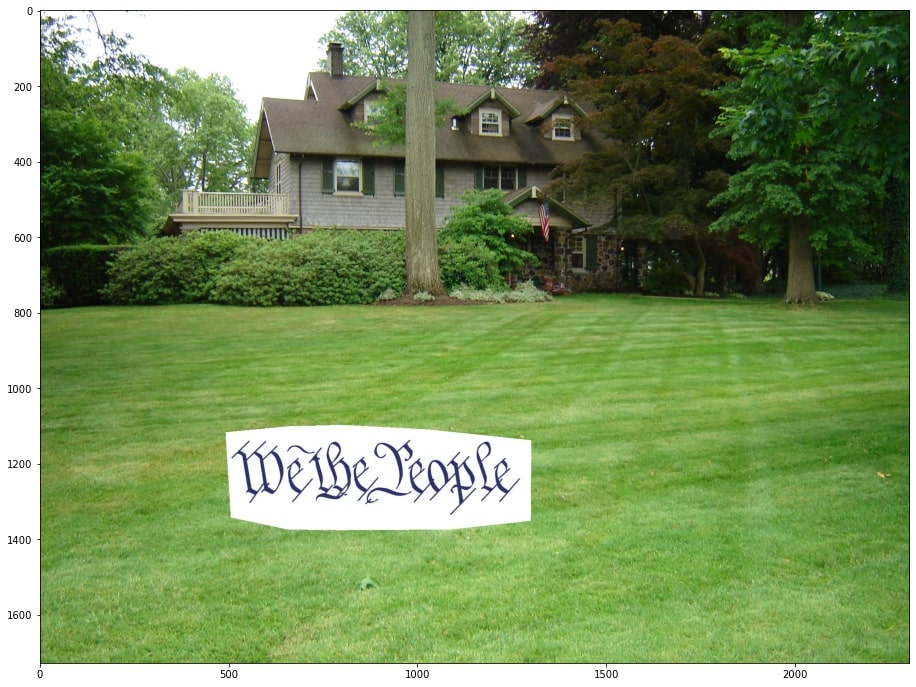
We first ask users to input 10 landmarks in the source image, which will be used as the vertices to construct a polygon around the source. We also give users to option to scale up or down the source before belnding. Next we ask users to input 1 landmark in the target image, which will be used as the location where the source will be blended into the target. We then naively blend the source into the target to see what it looks like.
Before setting up the system of linear equations, we first need to keep track of all the points inside the polygon. Then we iterate through every point inside the source polygon and look at its four neighbors: if the neighbor is also inside the polygon, we add a new equation corresponding to the first part of the given formula; if the neighbor is outside the polygon, we add a new equation corresponding to the second part of the given formula.
Unlike the toy problem, since we are blending two relatively large images this time, we have to take advantage of the sparse nature of the system of linear equations we are trying to solve; otherwise, our program will run for a long time and terminate when it runs out of memory. Luckily, SciPy gives us the tools we need. We then set up the system of linear equations to make the gradients match and solve it using least squares.
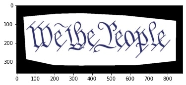
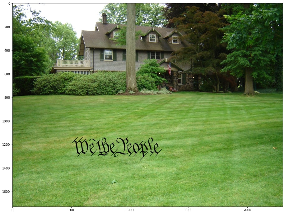
Since we are working with RGB images, we will work with each color channel of each image separately. We can see the second and the third examples look fine, but we see a rectangle boundary around the writing in the first image. Here are three examples on three rows:

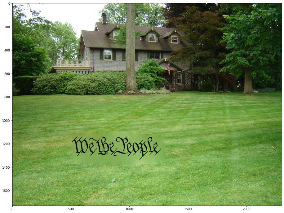

When setting up the system of linear equations corresponding to the first part of the optimization problem (points inside the polygon), instead of looking at gradients in the source only, we look at gradients in both the source and the target and pick whichever is bigger. We can see that this improves the writing on lawn blending a lot.
The following summarizes the algorithm proposed in the paper. The goal is to choose an input image to VGG19, which minimizes a linear combination of the content loss and the style loss. The style loss measures the similarity between the network’s output and the style image, while the content loss measures the similarity between the network’s output and the original image. The alpha-beta ratio is used to tune that linear combination, where a high ratio will weight the content loss higher, so the image won’t change as much.
The paper is fascinating because it demonstrates that neural networks allow us to differentiate between style and content in images.
The paper calls for us to minimize a linear combination of the style loss and the content loss using gradient descent. Hence, we used the Adam optimizer to minimize the loss. We start by creating a new neural network architecture which returns the feature representations of select layers during the forward pass.
To minimize the loss, we first choose an alpha-beta ratio. In the paper, they started with a white noise image, but after experimentation, we found it was easier to start with the original image. Hence, we pass the original image as a parameter to Adam.
Then, we run 300 training epochs on the original image, with a learning rate scheduler that decreases the learning rate on a plateau. Once the generated image is trained for a given alpha-beta ratio, and subset of layers, we only have to train for 150 epochs after changing those parameters.
In all images below, I used the same picture as the paper as the original content image. Here is a recreation of the plot from the paper, with the rows as Conv1_1, Conv2_1, Conv3_1, Conv4_1, and Conv5_1. The columns are 1e-5, 1e-7, 1e-10, and 1e-15, which are the alpha-beta ratios.

Below are results for the same paintings used in the paper, and you can see the results on Composition VII above. They show Starry Night, The Shipwreck of the Minotaur, Der Schrei, and Femme nue assise.


Here is an example using Der Schrei, and an image I chose. I show the original image first, followed by the result.


Overall, I was pleased with the results. They aren’t exactly the same as the ones in the paper, but the differences can be attributed to the use of different pictures, at different scales, different training methods, or different weights in the pre-trained model. As I ran the code, I realized that it was pretty unstable: the output changed a lot between runs. This is partially due to a high learning rate during training, but this made it challenging to produce results that were similar to those in the paper.