Overview
In this project, I played with different focus depths and apertures to focus on different areas of an image.
Given a list/directory of many images taken at different camera locations with different image centers, I calculated
the appropriate shift of each image such that aligning them at a factor would focus on different depths of the resulting image.
This was achieved by using the image centers to calculate the appropiate shift, multiplying by an alpha term to determine depth
focus location, and then averaging the resulting shifted images.
Depth Refocusing
For this part, I implemented depth refocusing using the method discussed in the paper. I noticed that every image
contained the coordinate of the camera's center location so I first averaged all of these points to determine the
true center of all the images. I then calculated the shift between every image and the calculated center average point.
To do different depths of focus, I multiplied this shift by a factor alpha of varying values from 0 to -0.5 and then
shifted all images by the calculated alpha * row shift and alpha * col shift.
Results:
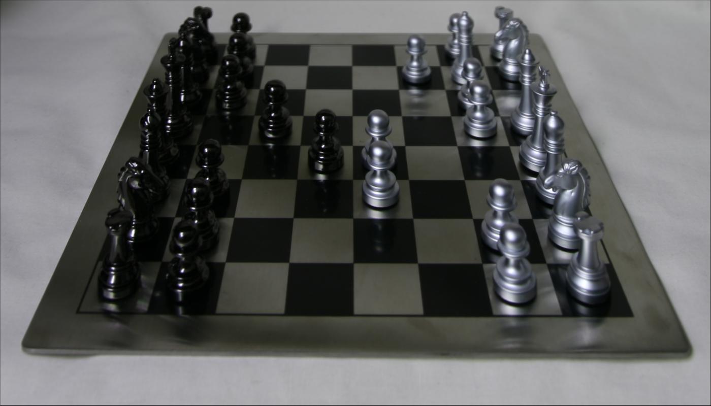
 Alpha = 0
 Alpha = -0.1
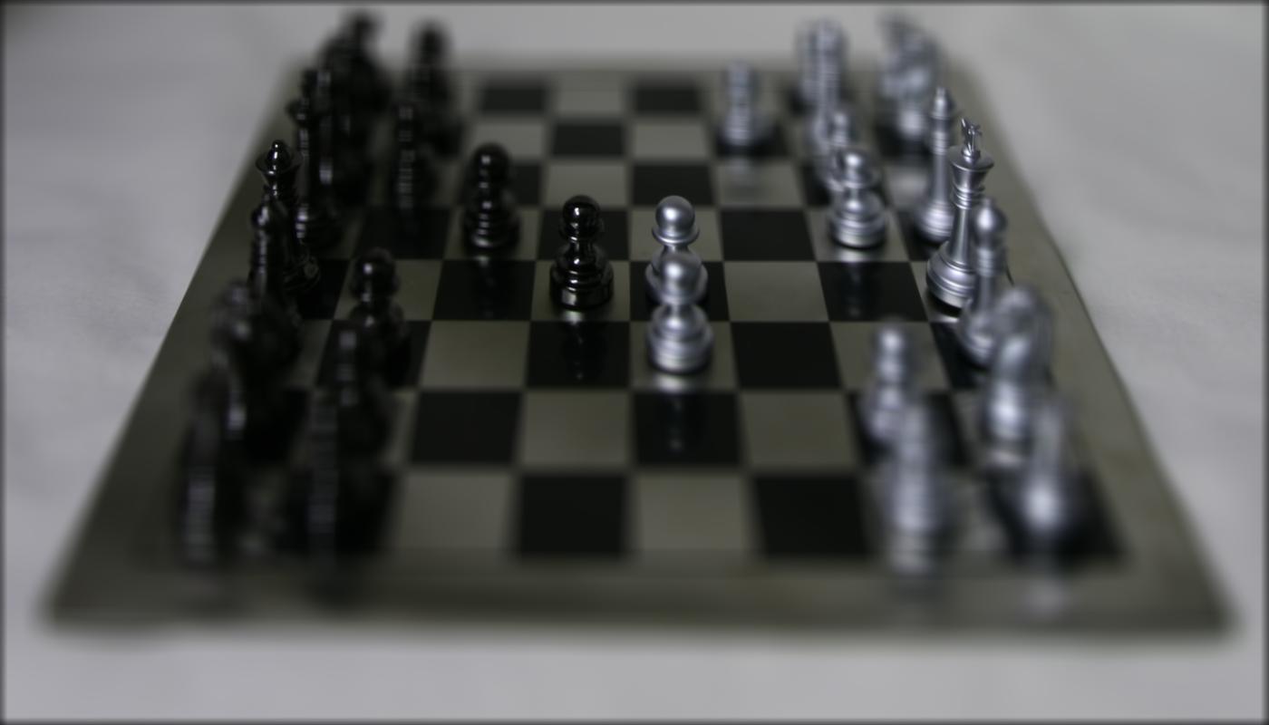 Alpha = -0.2
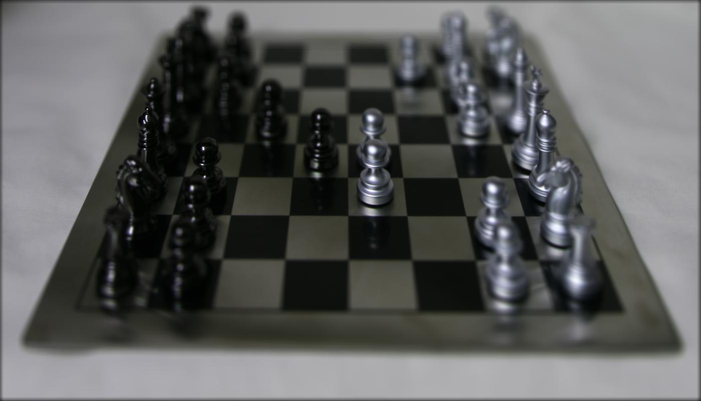
 Alpha = -0.3
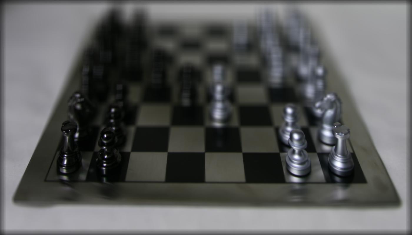
 Alpha = -0.4
 Alpha = -0.5
Gif:
Note: I performed shifting by making a very large grid and then placing the resulting averaged shifted
images at the appropriate offset. I then cropped out the excess to only take the original centered image region.
In this process, the shifted images cause a dark border to appear which gets larger for greater shift amounts (higher alpha).
This is completely normal -- I probably should have just cropped a bit extra to account for the largest shift but I didn't find that necessary for the exercise.
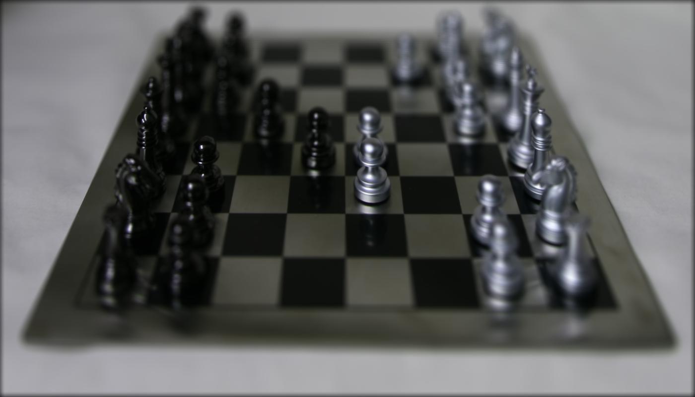
Apertures
In this part, I played with different focus aperture sizes by changing the amount of images I used when averaging.
The following results show the different focus aperture regions for various values of n where n represents the n closest
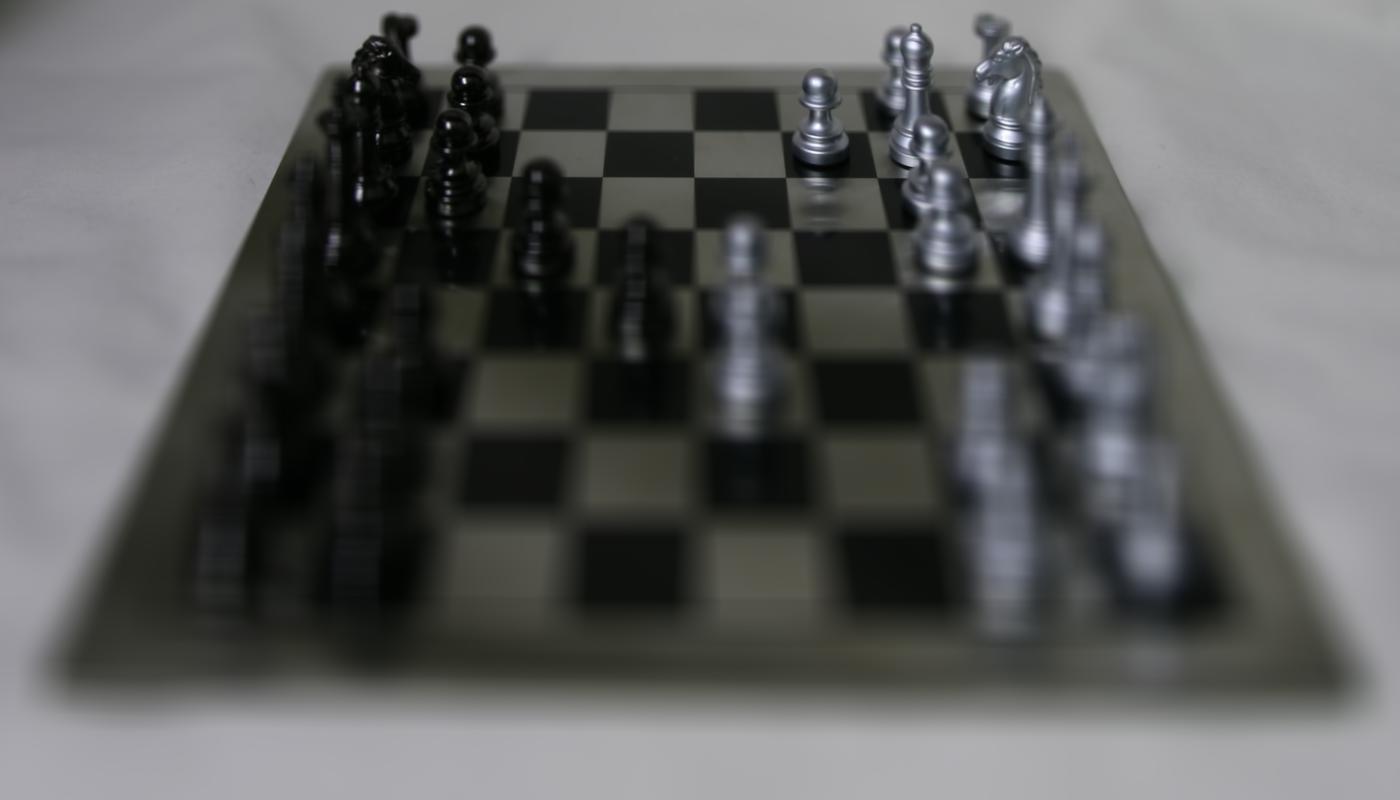
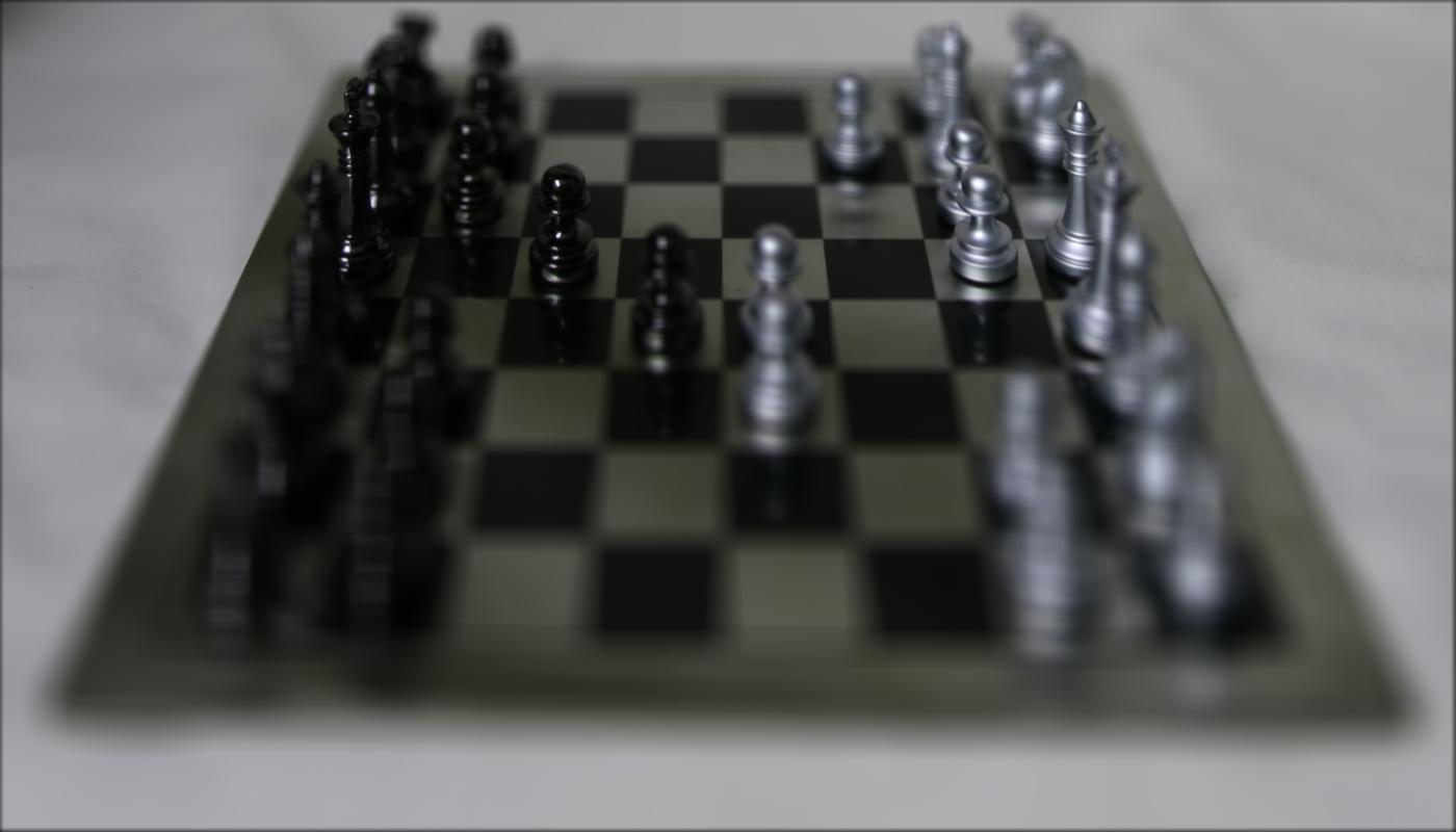
images (images with the smallest shift) from the center. All of the following results used an alpha value of -0.3 which
focuses on the center pawn of the image and you can notice the increasing blur especially in the corner chess pieces
as the value of n increases.
Results:
 n = 6
n = 6
 n = 56
 n = 106
 n = 156
 n = 206
 n = 256 (all)
Gif:
What I Learned
In this project, I learned a lot about how cameras work in terms of focusing on different regions of an image.
I thought it was really cool that implementing something like focus could be done simply by calculating image centers
and applying an associated shift to blur/focus different areas of the image. It was also interesting to learn that
the focus size can be adjusted simply by the number of images used in the averaging calculation.
Overview
In this project, I learned how to blend images using a least squares gradient fusion method. This method integrates
a source image into a target image by ensuring a least squares difference in the
source and target image pixels which propogates target image values inward toward the source image and creates a more realistic
integrated look.
Toy Problem
For this part, I implemented the least squares equations to solve the toy problem which
resulted in the same output result. The original and output images are shown as follows:
 Original
 Reconstruct
Implementation methodology:
For this part, I implemented the equations provided in the spec. I started by iterating through every
pixel in the image. For each pixel, I created two equations and assigned the appropriate values into the
A and b matrices. That is, for each v(x+1, y) - v(x,y) - (s(x+1, y) - s(x,y)) equation, I added a row in my
A and b matrices which contained a 1 and -1 at the column index corresponding to the index of the variables
v(x+1, y) and v(x,y) respectively and then added a row to the b array equal to s(x+1, y) - s(x,y). I then
stored a map containing all the mappings in both directions from the variable v(x,y) to its assigned index
in the column of A. Finally, I added one final row which just contained a 1 in the first column (corresponding
to v(0, 0)) and s(0,0) in the b array for the uniqueness guarantee of the same color shade. I stored A as a
scipy sparse matrix by only keeping a list of values (1's and -1's) and corresponding lists for the row and column
indexes corresponding to each of these values.
Poisson Blending
For this part, I implemented poisson blending where I blended each source image
onto the target image. Here are some results of various blendings.
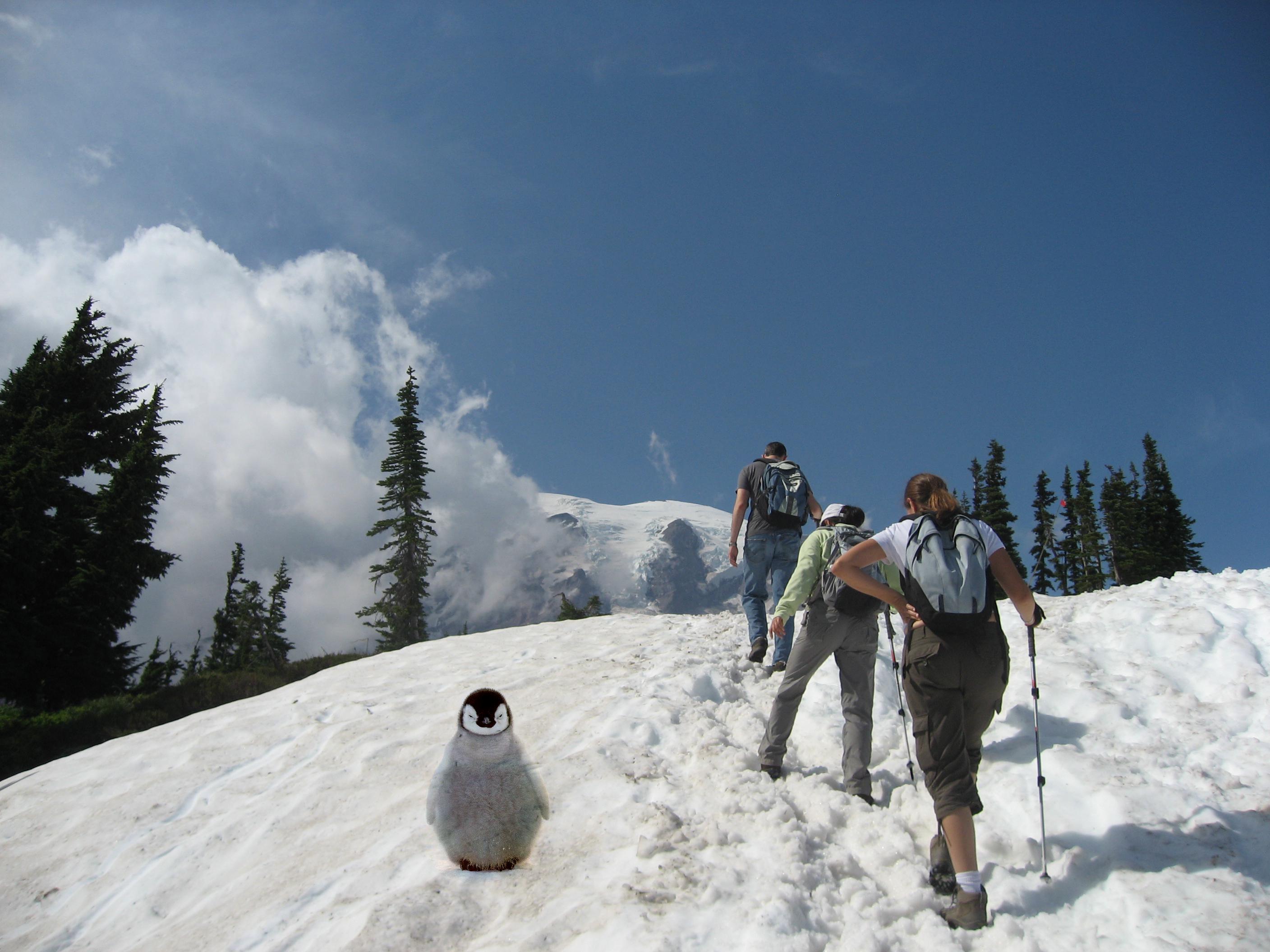
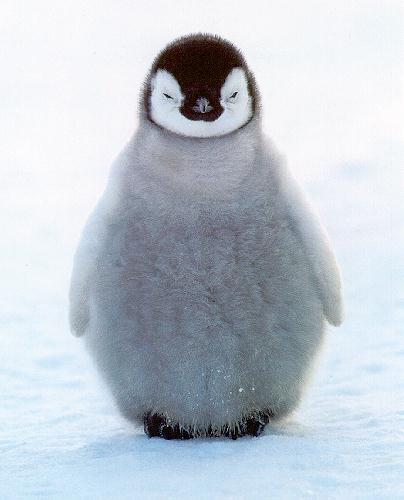 Original penguin
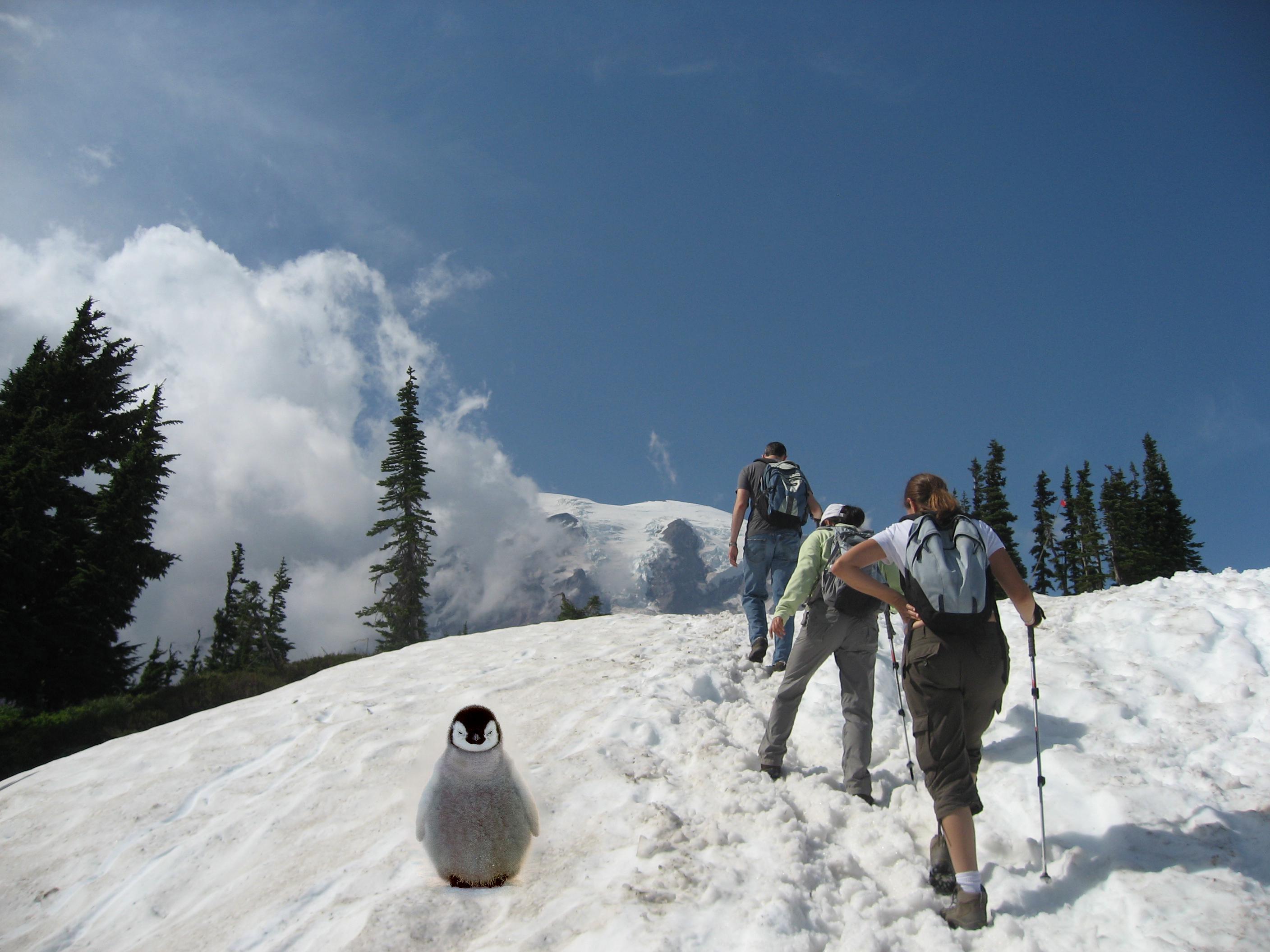 Blended image
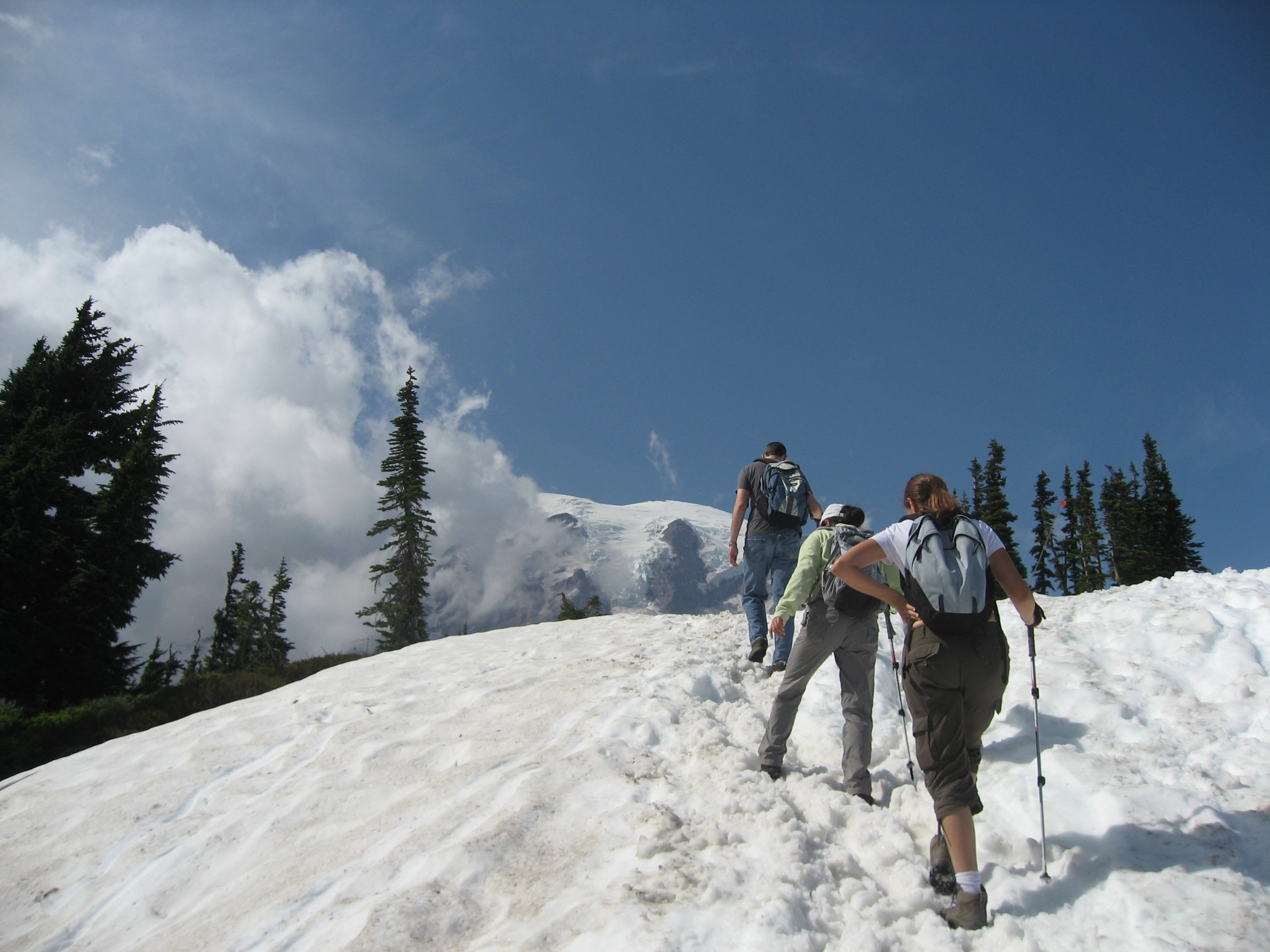 Original Skiers
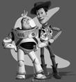
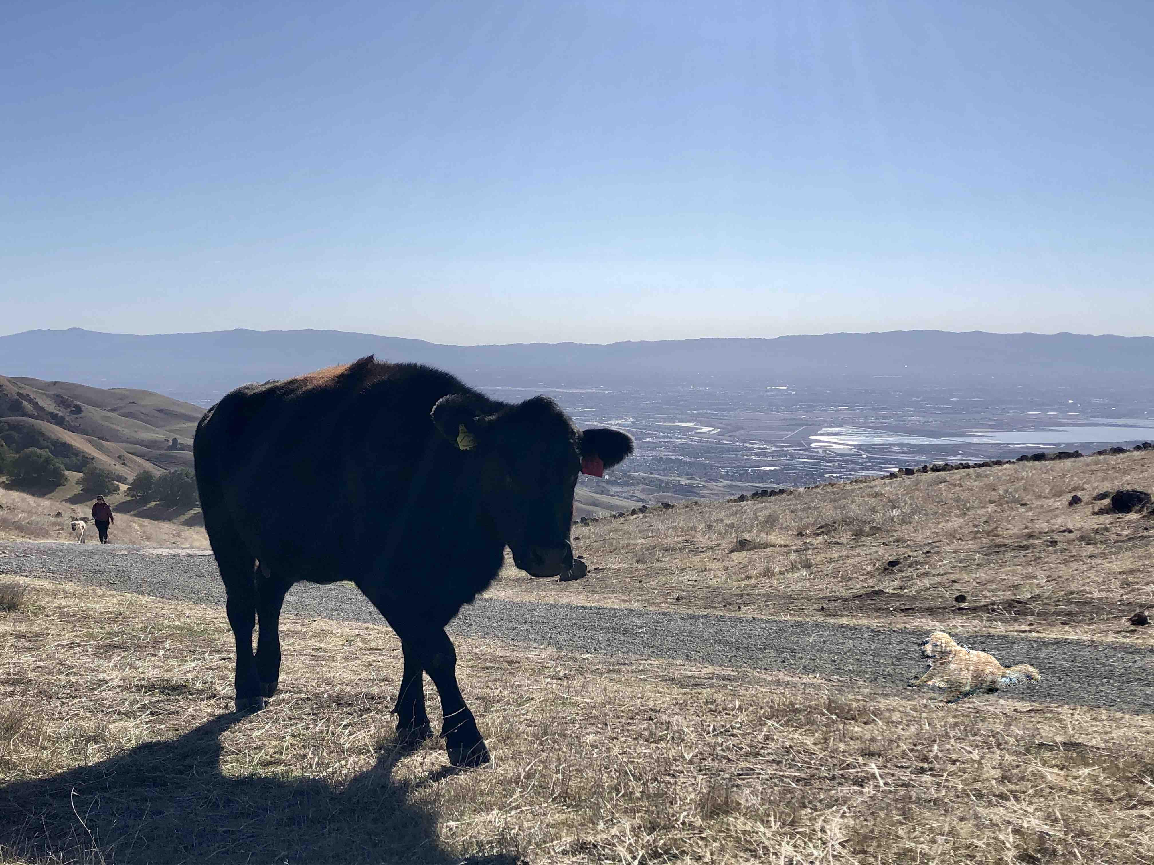
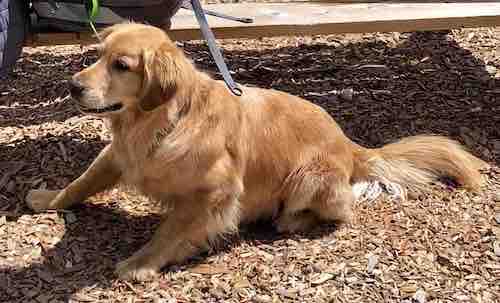 Original dog
 Blended image
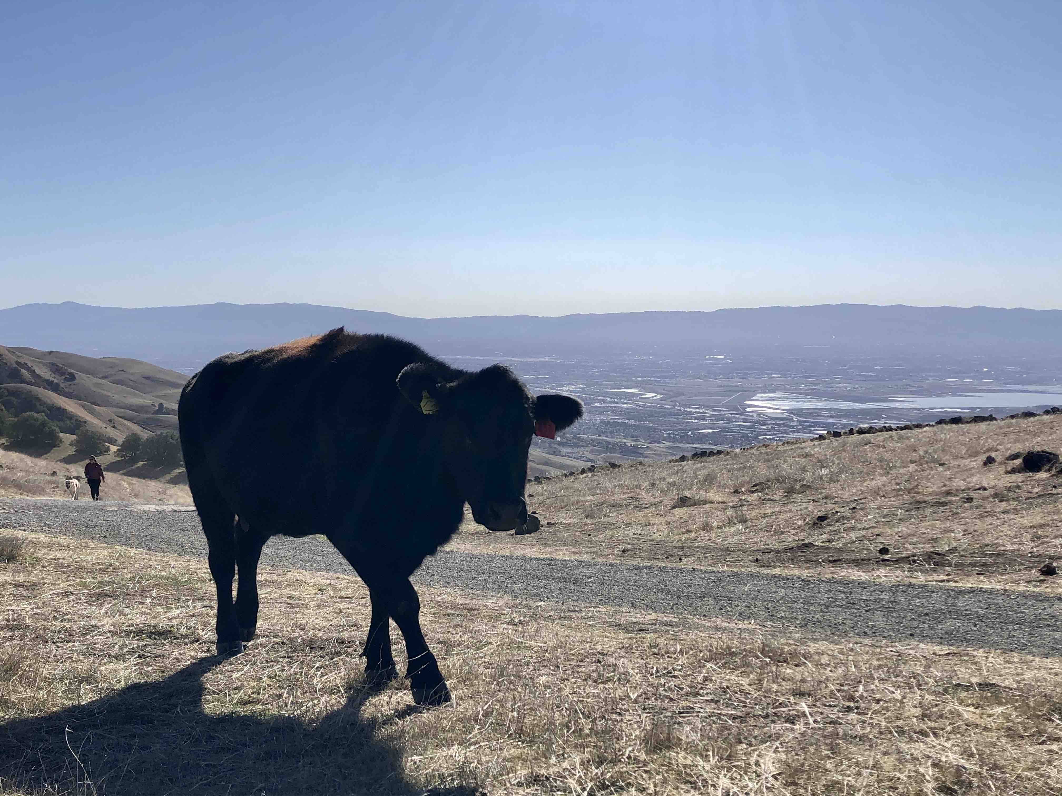 Original Cow (on Mission Peak!)
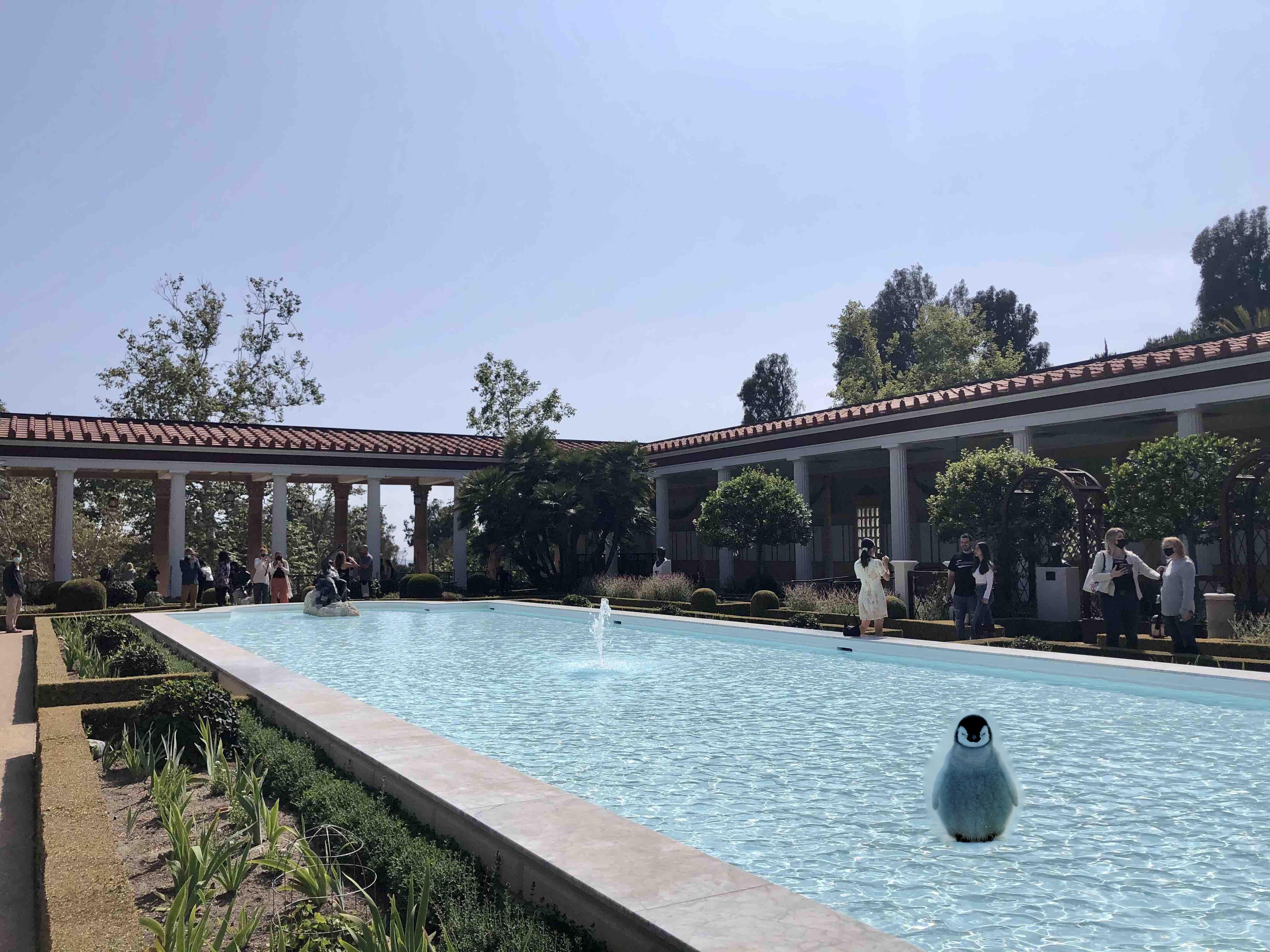
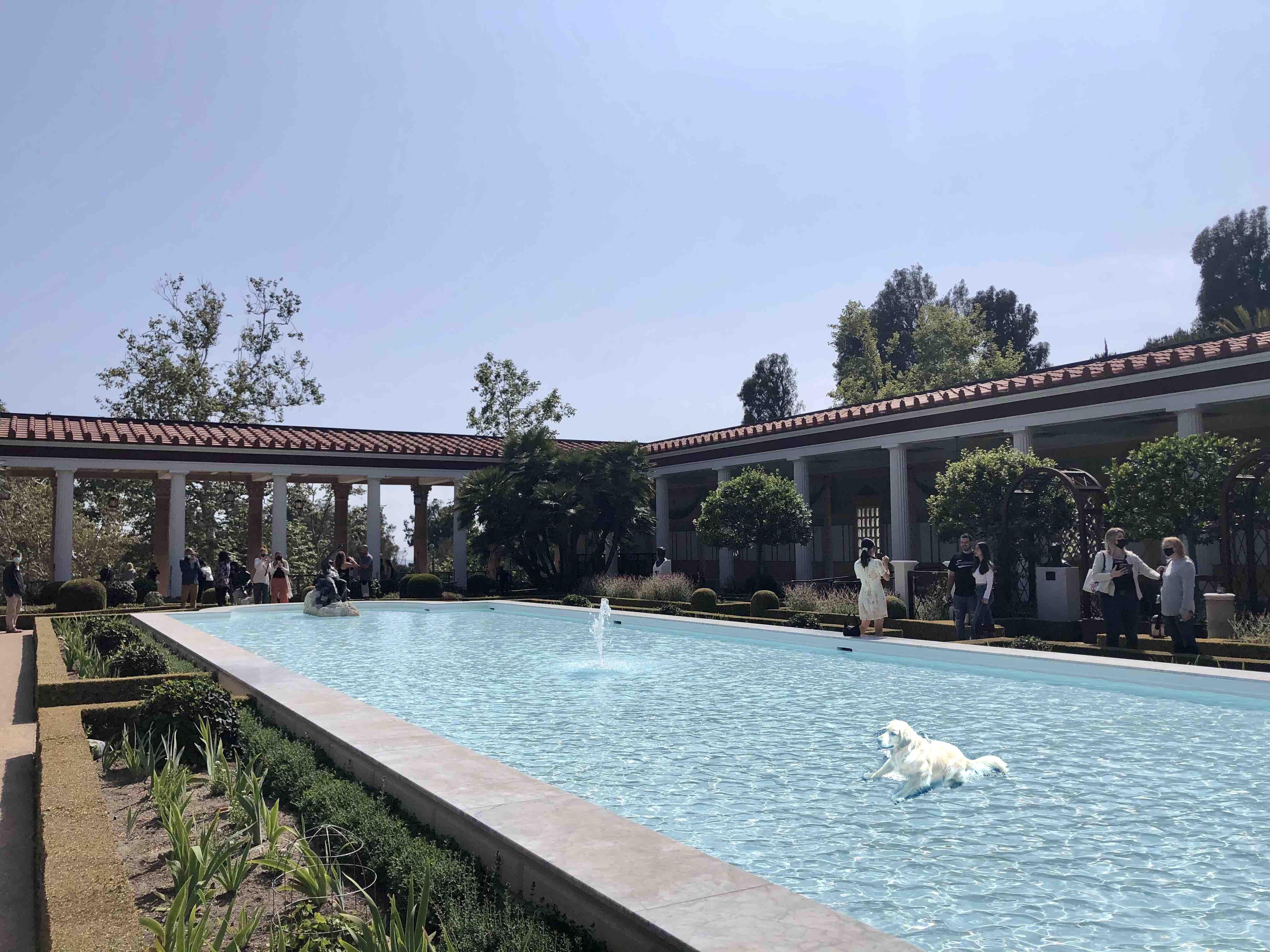
Here are also some examples of unsuccessful images. Taking inspiration from the dog swimming
image in the spec, I wanted to see if I could also place my animals on water and make it appear as
if they were swimming. The results didn't work well since neither of the source images were underwater
so the lighting and general blended edges did not match the water. The result is that a lot of the water
shading ended up being blended through the entire image and the penguin looked like it was underwater and
the dog looked like a ghost dog (or a dog shaped splash?)
Original penguin
 Blended image
 Original pool
Original dog
 Blended image
Original pool (from the Getty Mansion!)
Implementation methodology:
My implementation for this part was very similar to the previous part but with some slight additions.
To start off, I implemented my own masking code by creating a select points method that allows the user to
select a series of points and then using the ImageDraw polygon function to create a polygon
mask. I then prompted the user for a point in the target image which would serve as the top-left corner of the
blending region. The actual creation of the A and b matrices was very similar to the previous part, except instead
of iterating over the entire image, I iterated over only the masked region. I again created a mapping of
variables to column indices of A and created a sparse matrix by recording the value coefficients (1 or -1) and
the row and column indices for each point. The b matrix was formed by subtracting the adjacent pixels of the source matrix.
I did this over all three color channels separately and then one-by-one replaced the masked region on the original
image with the new calculated values after my least squares for each color channel.
Bells & Whistles
For the bells & whistles, I implemented mixed gradients which used the larger pixel value difference between source vs target image as the b value in the b matrix rather
than always using the source difference. I found that this improved the image in some cases but not in others. Here are the results
on my two well-performing images of the previous part.
Normal gradient fusion
 Mixed gradient fusion
Normal gradient fusion
 Mixed gradient fusion
From the results, we can see that the penguin image performed much better as the background region
around the penguin where I cut out the mask is a lot more integrated in the mixed gradients case. This is
likely because the mixed gradient successfully identified that the prominent feature in the cutout borders should
be the target background so more of the target background was incorporated there. For the dog image, due to
image sizing and resolution issues, the target image ended up having a lot higher resolution which resulted in greater
pixel-neighbor differences so using the mixed gradient actually made the dog seem a bit translucent since it was
sometimes using the target background for regions in the middle of the dog where the background had a lot more
gradient movement than the dog's fur in the foreground.
What I Learned
In this project, I learned a very cool method of blending images that was different from the Laplacian pyramid
method which I thought was cool since this one better integrated an image by enforcing a least squares difference
along the border of both images rather than just creating a smooth gradient blend. It was really interesting to see
how linear algebra equations could be applied to make really interesting and natural looking blended results!