Reimplement: A Neural Algorithm of Artistic Style
Part 1: Algorithm Overview
In this project, I reimplement the algorithm mentioned in "A Neural Algorithm of Artistic Style" to utilize Convolution Neural Networks to combine one style image and a content image to produce a new image with similar content with the content image but artistic features from the style image. To be more specific, we utilize one convolutional neural network to extract the features from the style image and content image and then combine them into a single loss function that enforces the output image to have a similar style representation to the style image while not diverging too far from the content image.
Part 2: Neural Model
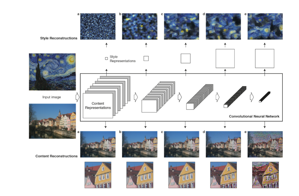
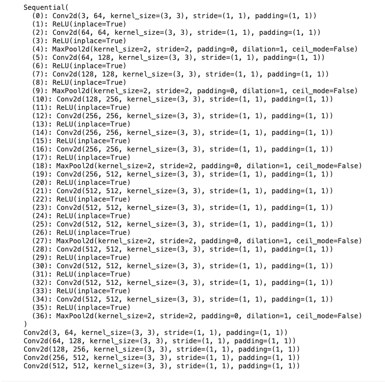
As suggested in the paper, we utilize a pre-trained VGG19 and use different convolution layers to capture features from the content and style images. As the paper suggests, I use 'conv_1_1', 'conv_2_1', 'conv_3_1', 'conv_4_1', 'conv_5_1' to compute the style loss, which is layer_0, layer_5, lay_10, layer_19, layer_28 in the model graph; also, I use 'conv_4_2' to compute the content loss, which is lyaer_21 in the model graph. As the loss term requires the intermediate results after these different convolution layers, I implement a forward hook to directly get intermediate results from the pre-trained model without access to its structure. Moreover, as the paper does not mention the input image size, I resize both content and style images to 224, which is the size VGG19 is trained. I normalize both image data with ImageNet's mean and standard deviation.
Part 3: Loss Terms
We need to introduce two types of loss to get great results: content loss and style loss. The content loss prevents the output image from becoming too different from the original content image. The style loss ensures the overall art features of the result are similar to the style image.
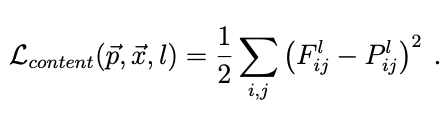
As shown above, the content loss is the sum of the square difference between F_l and P_l, where F_l is the content feature from the output image, and P_l is the content feature from the content image.
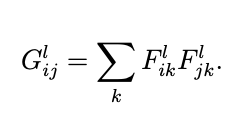
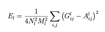
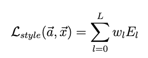
We first need to calculate the Gram Matrix for each layer's features for the style loss, which is a matrix multiplication product of F_l with itself. Because we use multiple intermediate results from the VGG19 to compute the style loss, we need to calculate the loss for each layer as E_l, which is the sum of the square difference between G_l and A_l. G_l is the style representation of the l layer in the output image, and A_l is the style representation of the l layer in the style image; both A_l and G_l are computed through Gram Matrix. After that, the style loss is the sum of different E_l with weight w_l. For my implementation, I made some modifications to the style loss: I didn't normalize the E_l, but for each w_l, I used 1 / (C_l * C_l), where C is the number of channels for each convolution kernel, such as 64, 128, 256, etc.
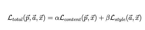
The total loss is the sum of content and style loss, weighted by α and β. For my implementation, α = 1 and β = 1e5.
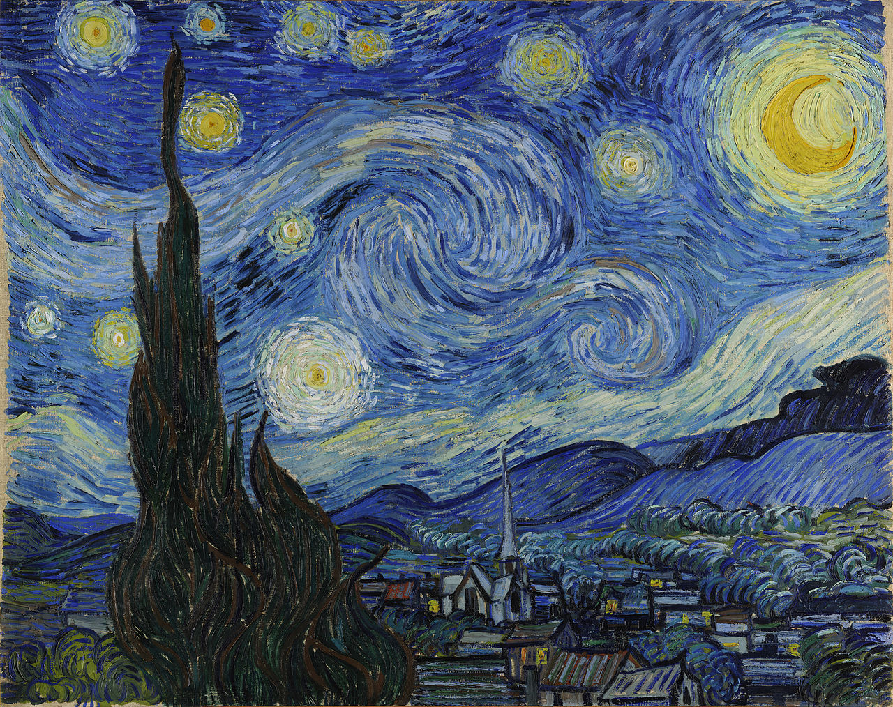
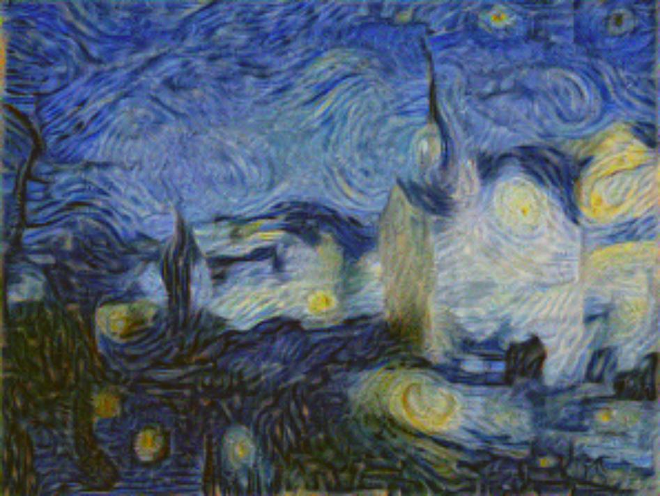
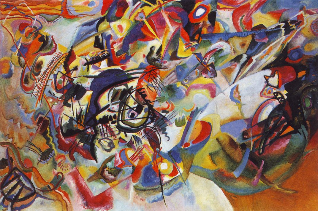
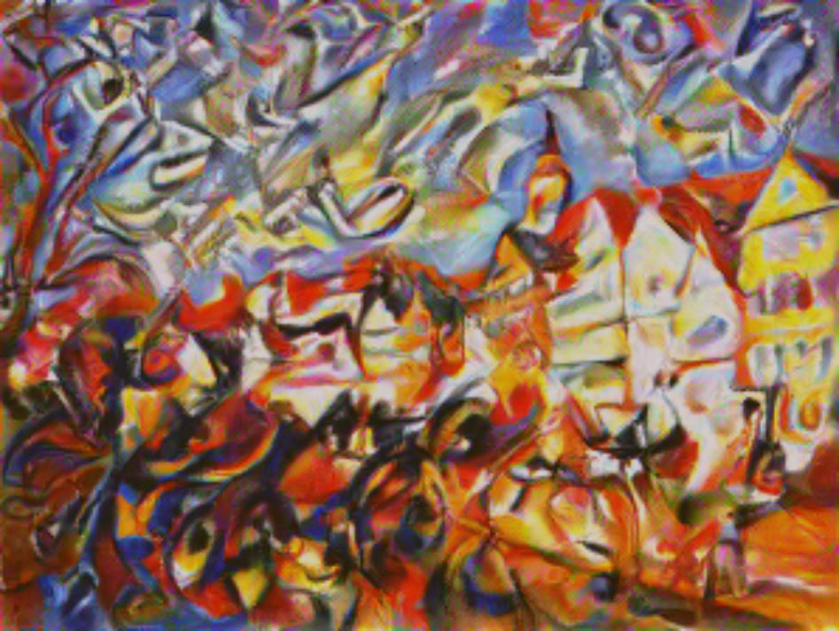
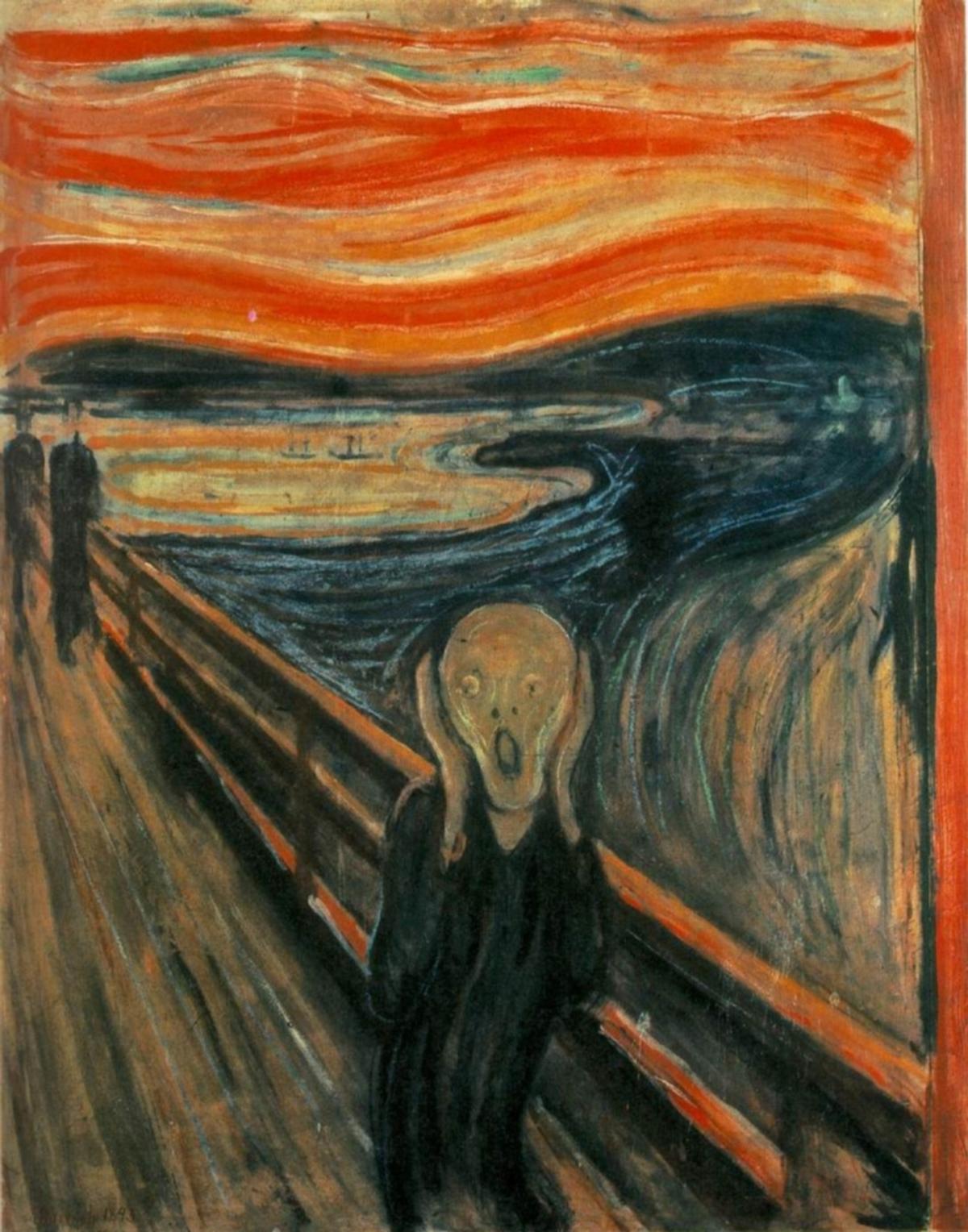
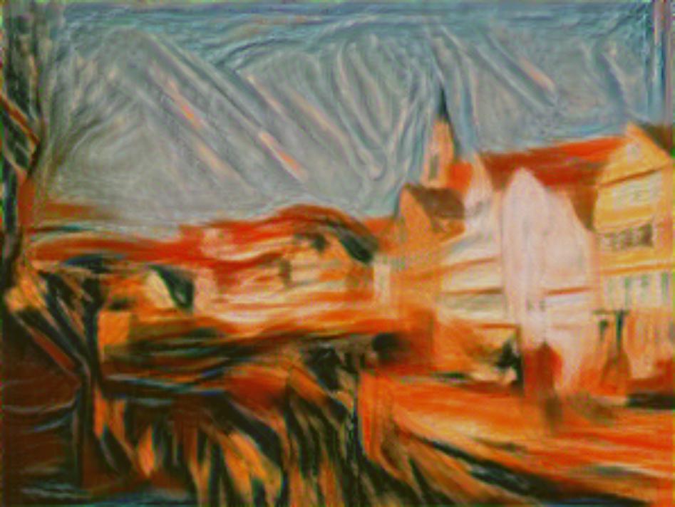
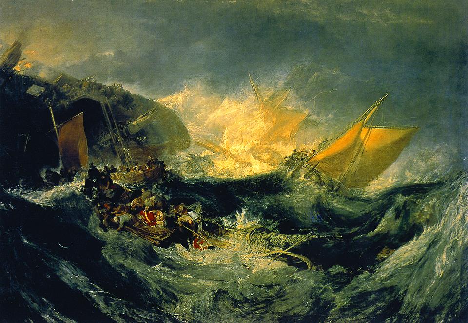
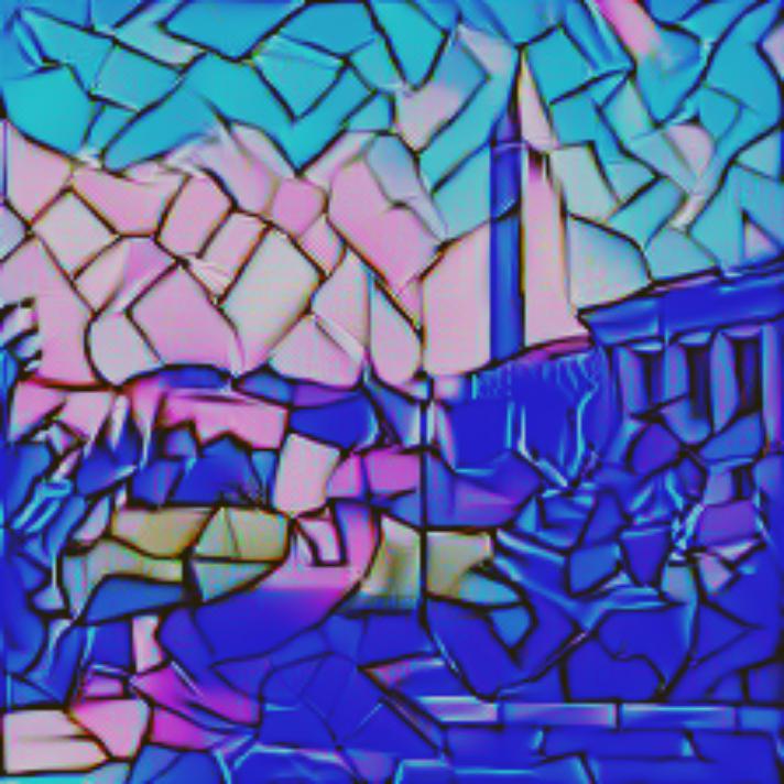
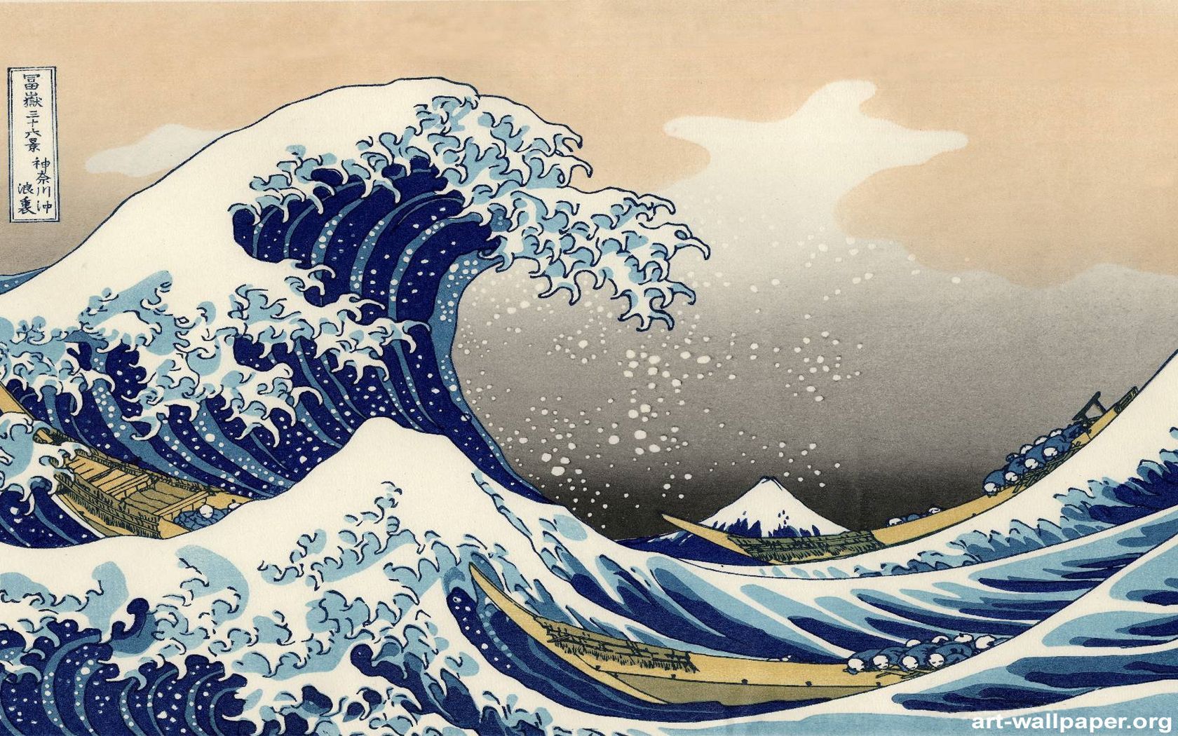
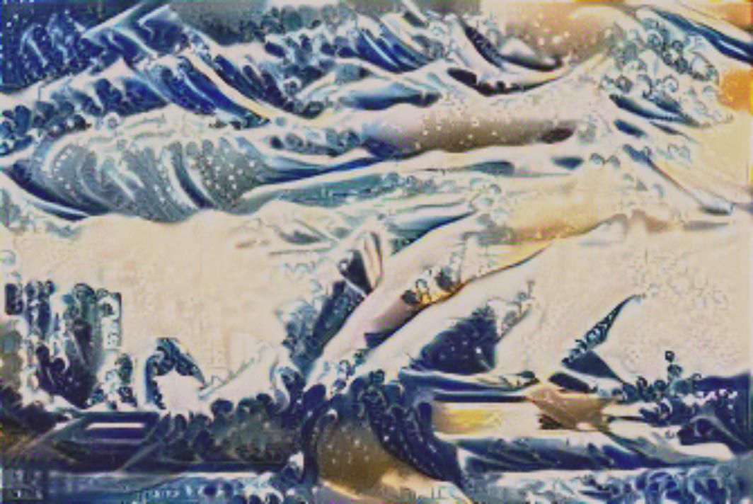
Part 4: Results from Paper's Images
In this part, I will share some reproduction of results from the paper. Notice that the performance of this implementation is very susceptible to different parameters, and I'll list all parameters I used for each result.
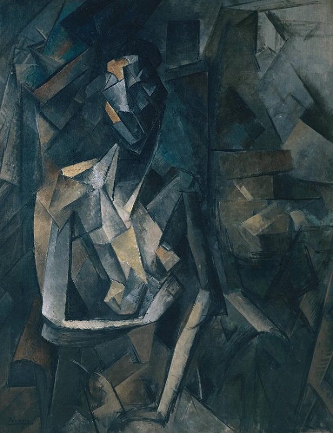
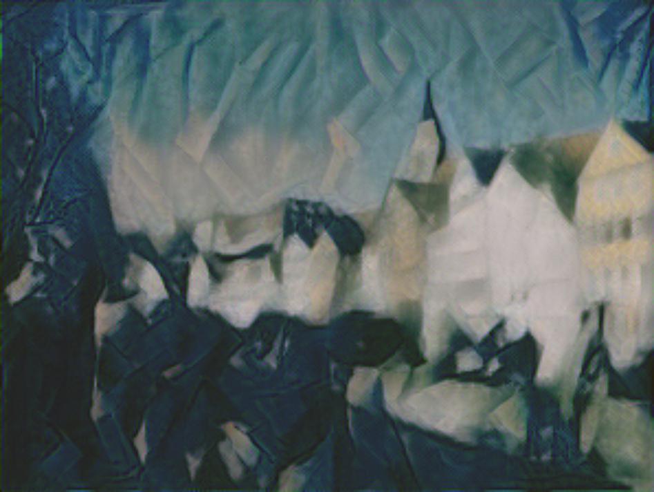
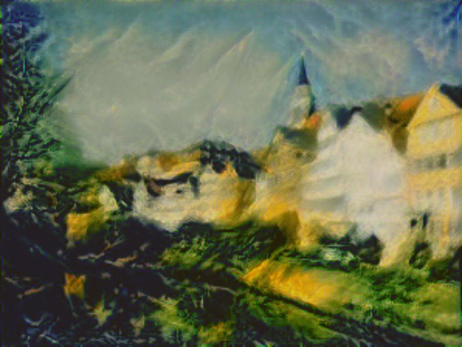
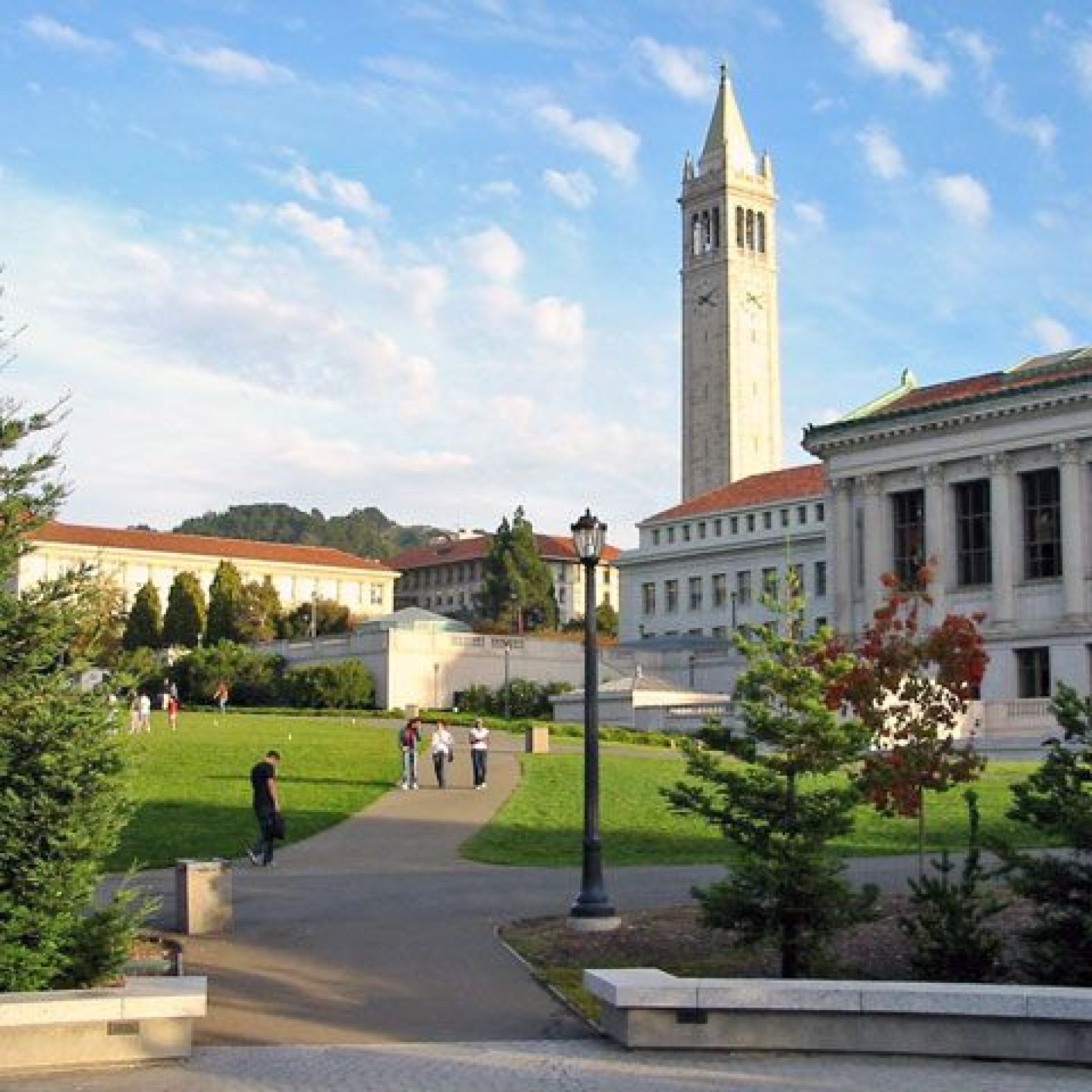
Part 4: Results from Self-Selected Images
In this part, I will share some results with my images.
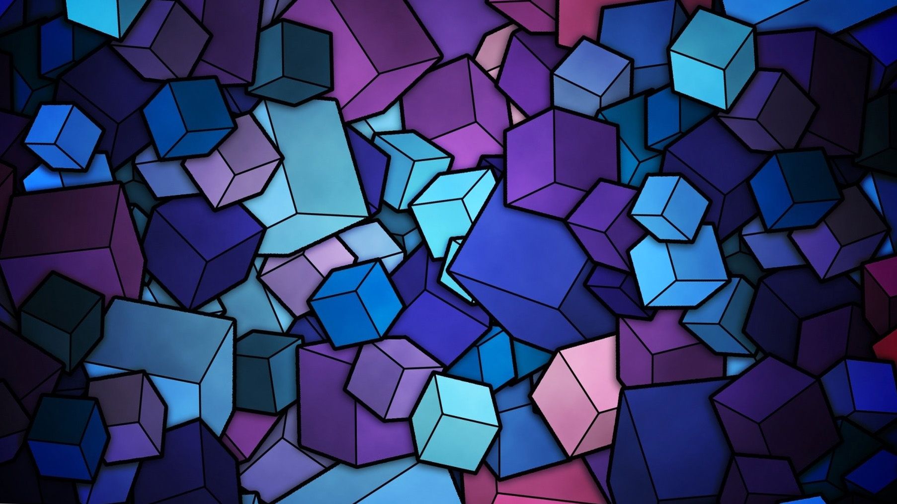
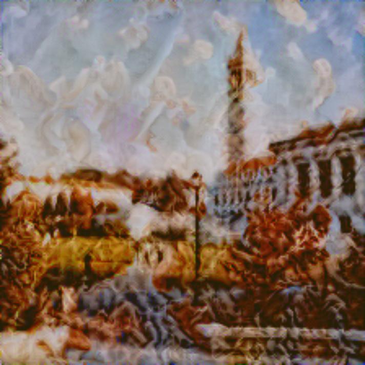
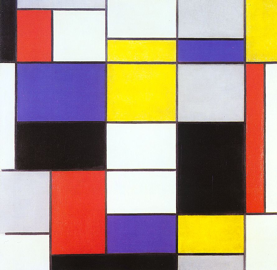
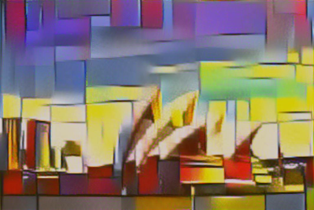
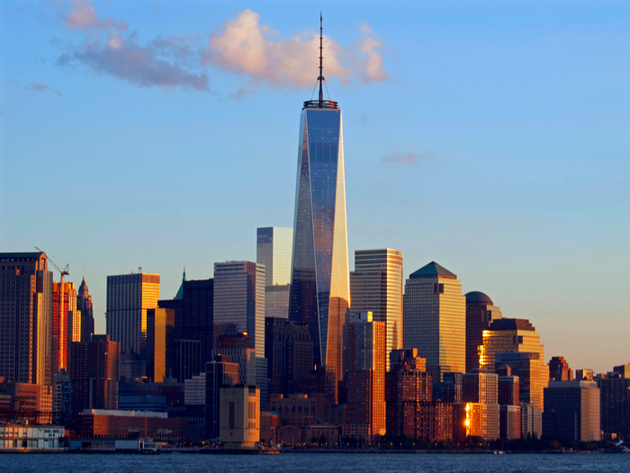
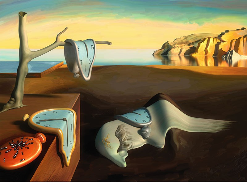
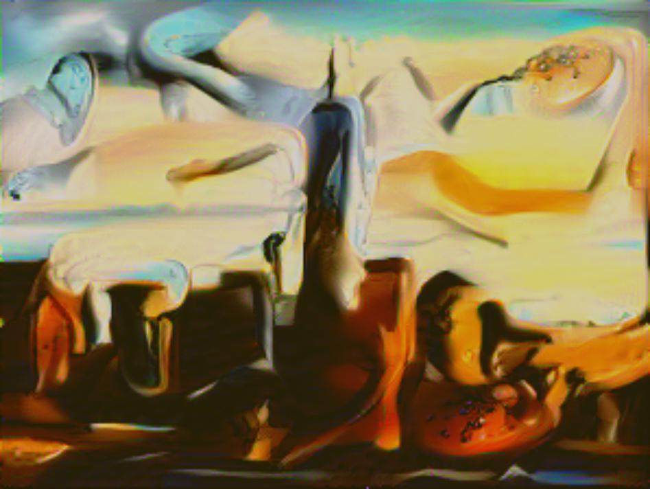
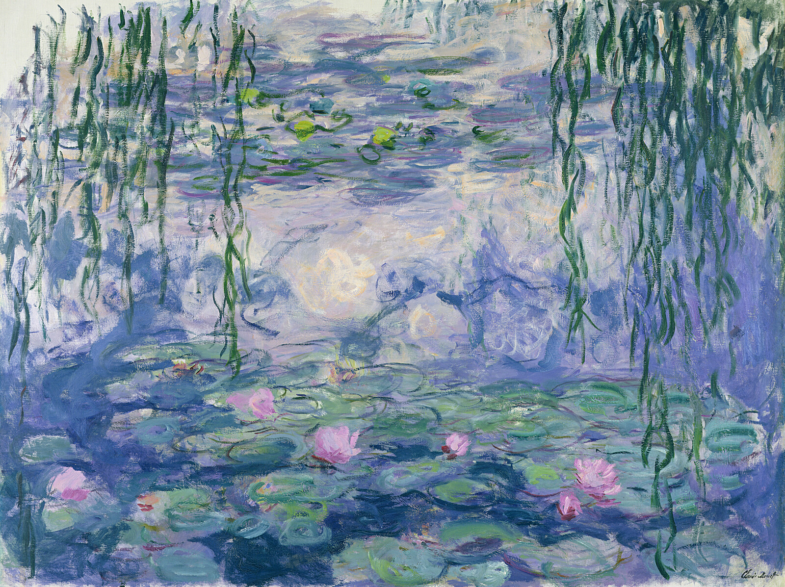
Generally, I found out that for style images with simple patterns, such as the Mondrian art, the Purple Cube, the Seated-Nude from Picasso, the learning rate should be lower, and the training epochs should be smaller. Otherwise, the image will look very different from the content image. On the contrary, if the style images contain some complex patterns, such as Starry-Night, the learning rate should be larger, and the training should be longer. Also, if the style images are not very stylish, the Neural Network cannot provide enough guidance for the output image, and the result would be random rainbow color gradients all over the image.
Gradient Domain Fushion
Part 1: Toy Problem
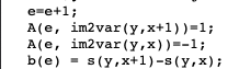
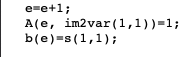
I implement a simple algorithm utilizing image gradients and linear least-square solutions in the first part. To reconstruct the images, we add constraints as the hint suggests to ensure that the x-direction and y-direction gradients are close to the corresponding points in the original image. Also, to ensure that the overall color is similar, we want to add one more constraint on the top-left pixel of the image. After adding all these elements to the A matrix and b vector, we use SciPy's least-square solver to get the output and then reshape it into the 2D image. As expected, the two images look highly similar.

Part 2: Poisson Blending
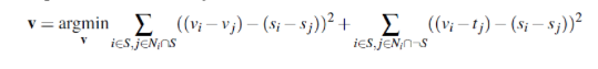
For the actual Poisson Blending, I would first get a pair of images, the source image, and the target image. Also, I'll need to draw the mask on the source image to indicate the region that I want to blend. Also, to simplify adding images, I need to select the place in the target image and shift and align the source image and mask image. I reused some codes from Our Proj2 and Proj3 to accomplish this.
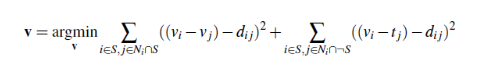
After getting all of these images together, the next thing is to construct the corresponding A matrix and b vector and utilize a least-square solver to get the results. This is an implementation of the formula shown below with the following steps: for each pixel, if it's outside of the mask, it should be directly the pixel from the target image; if it's inside the mask, then we need to add source image pixel to the constraint. Moreover, for these inside pixels, I need to add more constraints corresponding to the formula: if the pixel's neighbor pixels( up, down, left, right) are also in the mask, I add [-1] to the corresponding location of A matrix and update the b vector with source_img[ current pixel ] - source_img[ neighbor pixel], which is corresponding to the first half terms of the formula. If its neighbor pixels are not in the mask, I only update the b vector by source_img[ current pixel ] - source_img[ neighbor pixel] - target_img[ neighbor pixel], which corresponds to the second half terms of the formula. All of these ensures that pixels outside the mask have similar gradients to the target image, and pixels inside the mask have similar gradients to the source image. Those on edge inside the mask would become the fusion parts due to the second half of the formula.
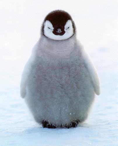
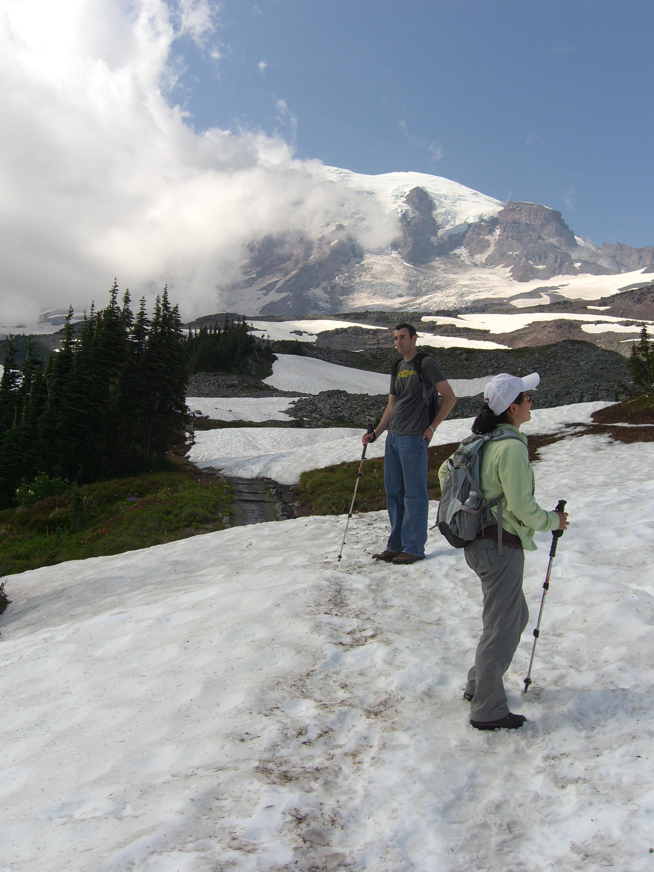
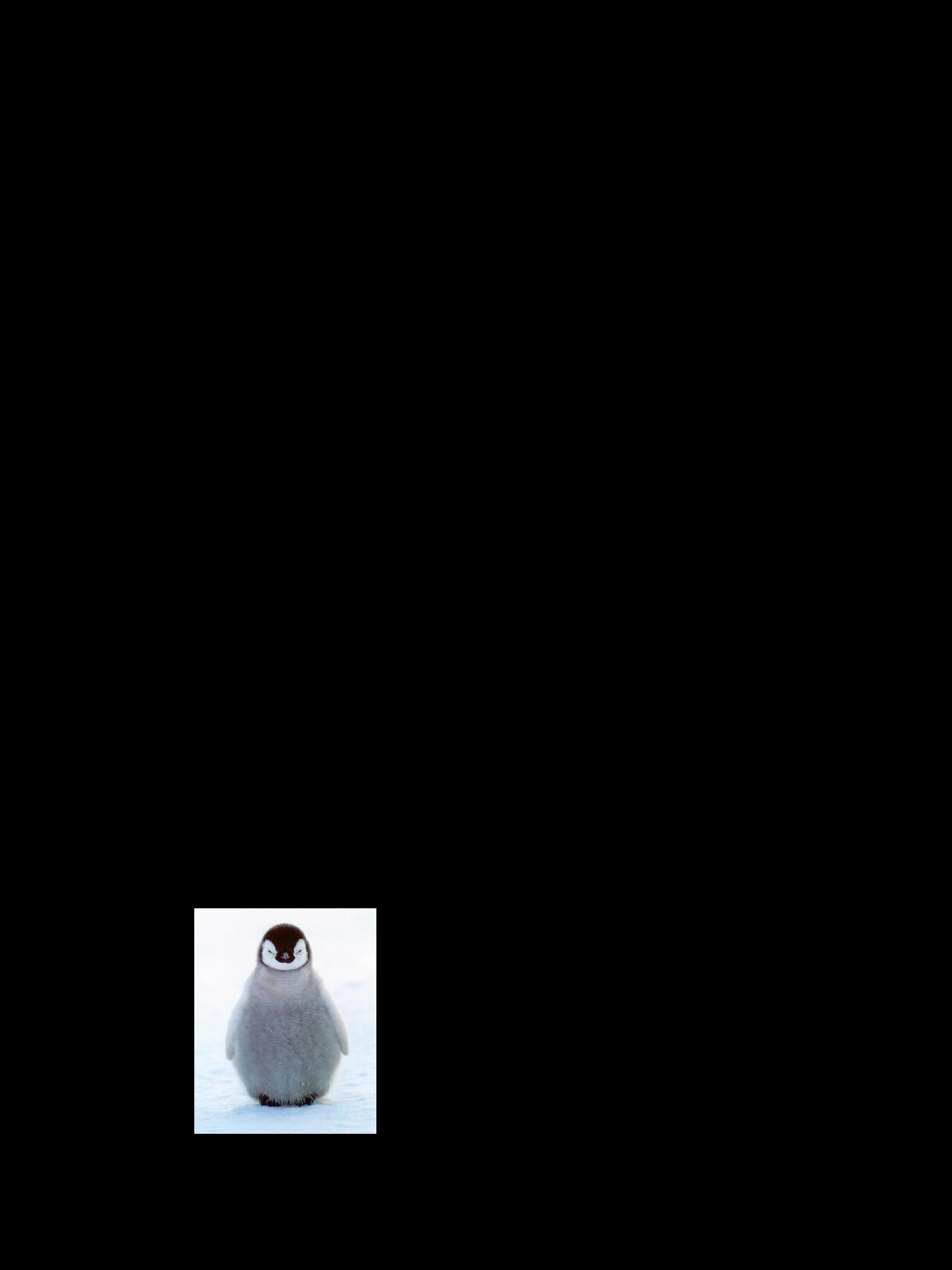
Here I want to share the penguin and the snow mountain results.
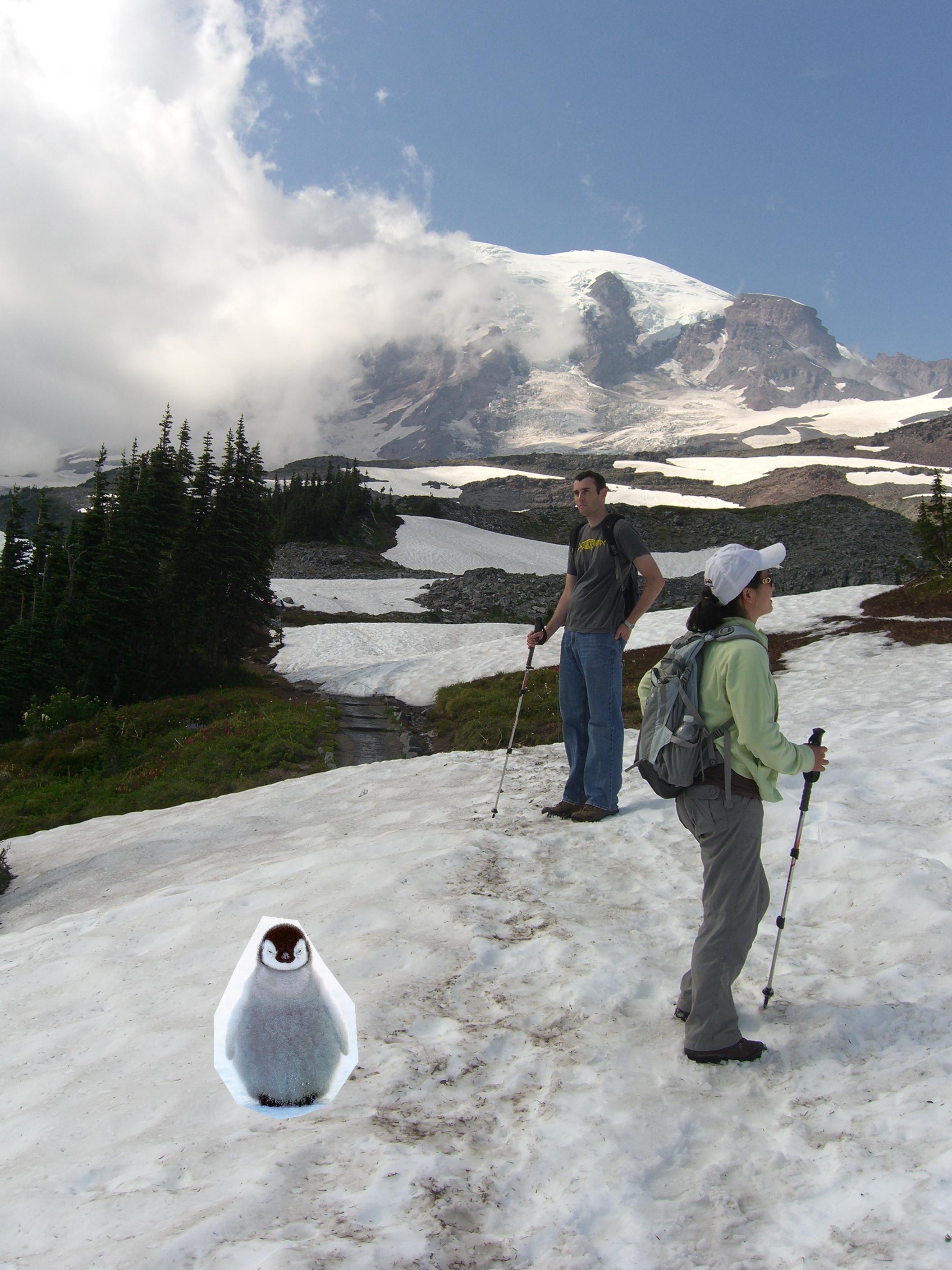
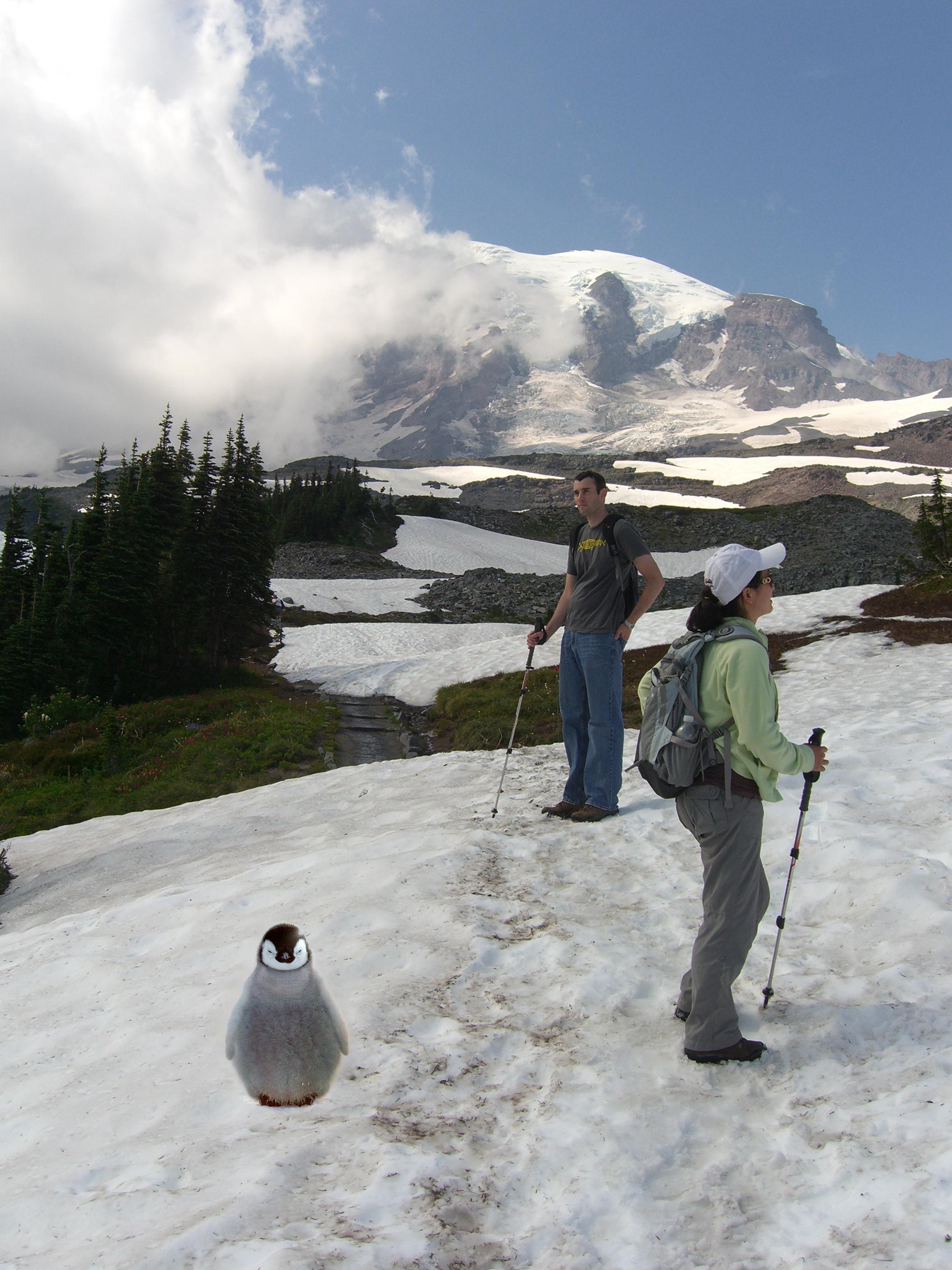
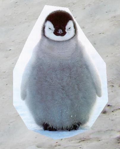
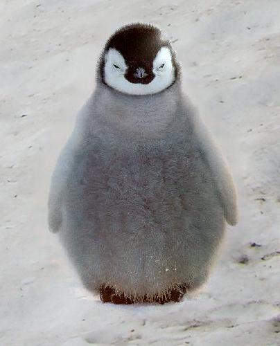
As shown in these graphs, the boundary in the direct copy ones is extremely noticeable, but the ones from the Poisson Blending are more realistic and smooth.
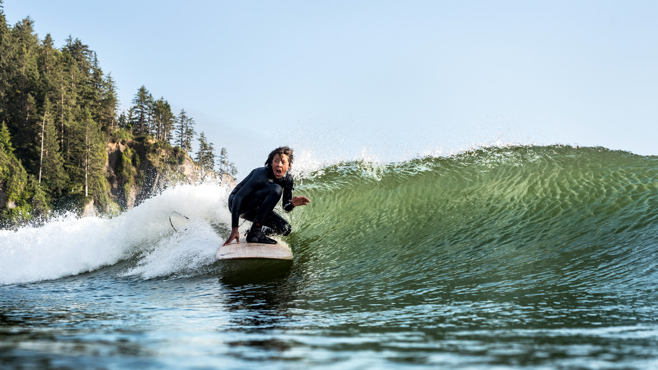
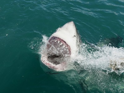
Here comes more examples:.
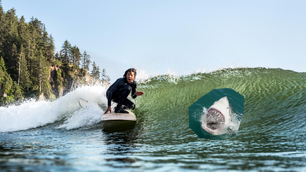
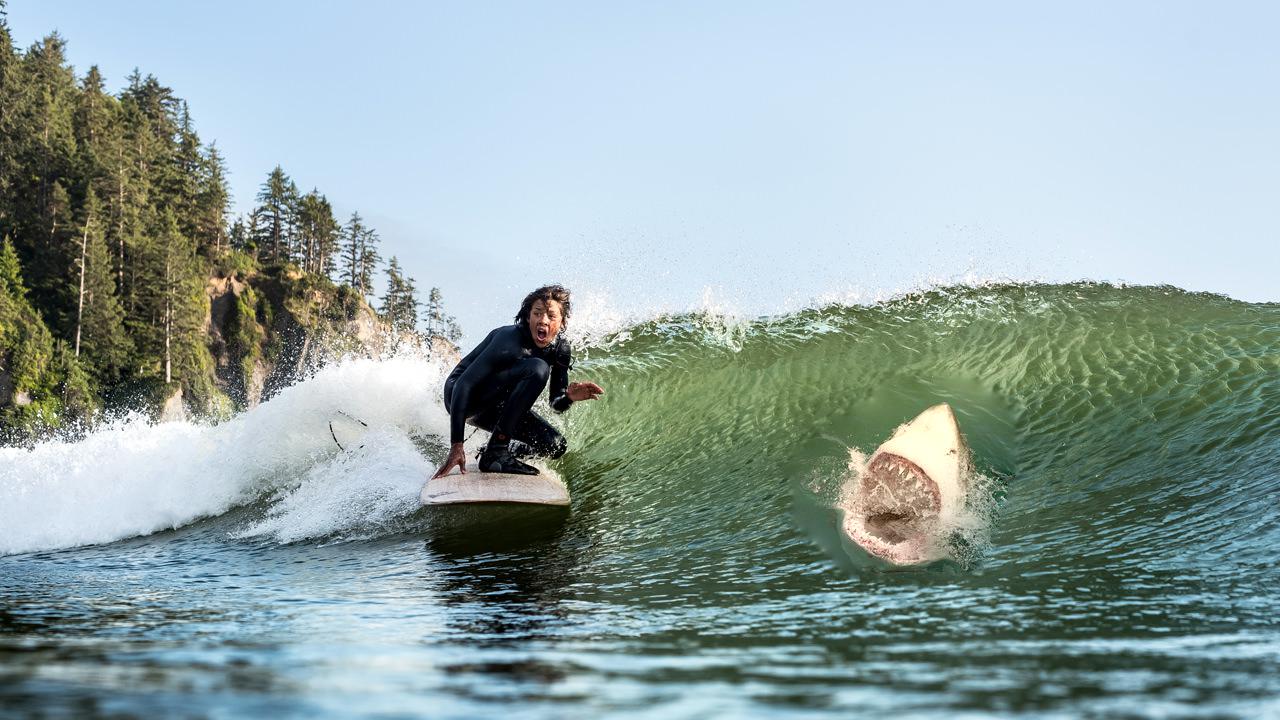
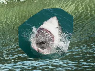
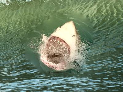
Shark in the surfing
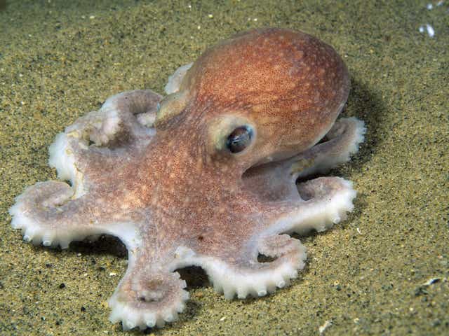
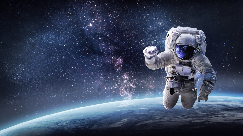
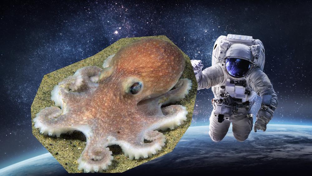
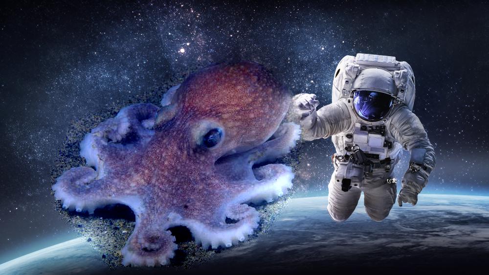
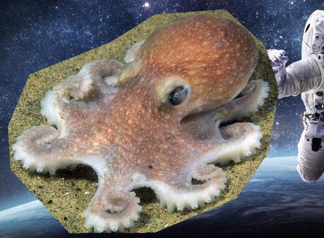
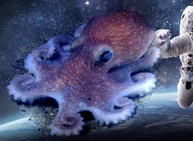
Octupus in the space
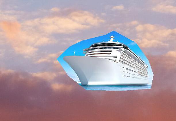
Ship in the air

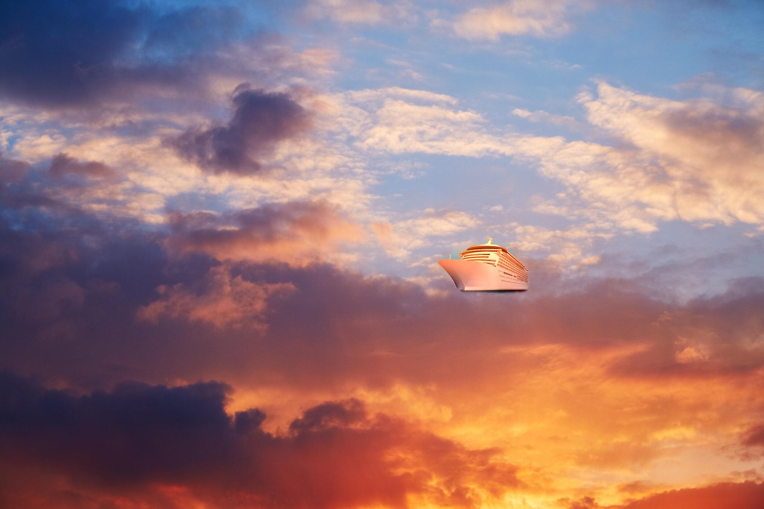
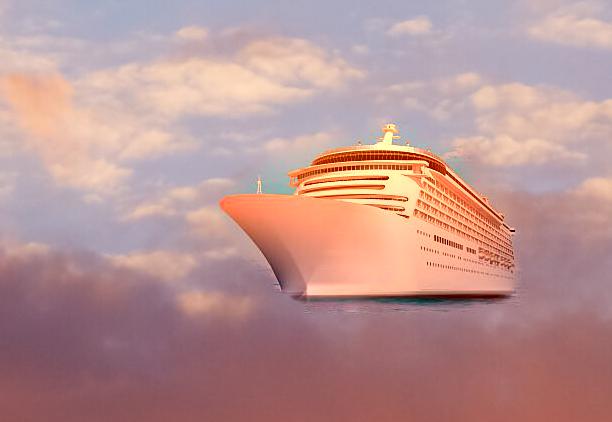
Notice that some blendings are still kind of unrealistic: for example, in the ship and sky case, the ship's color is bizarre from its nearby background; in the octopus, the structure of the bottom sand still exists in the space. I suspect that the color and the features(pattern) from the background of both the source image and target image for the Poisson Blending should be similar, otherwise even though the gradients' guide, the blending cannot be realistic as the case as in penguin and shark.
Part 3: Bells & Whistles: Color2Gray
In this part, I implement a fusion between the mixed gradient and the toy problem algorithm: for each pixel, add the constraint of the grayscale intensity and the corresponding stronger gradients from S, V channels in the HSV version of the image. At first, I tried to add the gradients constraints of H, S, and V channels, but the Hue channels change always leads to weird results. Below is the comparison of direct Color2Gray and Poisson Blending based Color2Gray.
Part 4: Bells & Whistles: Mixed Gradients
In this part, I modify the original Poisson Blending Algorithm according to the following formula. The only change is that instead of adding source_img[pixel] - source_img[neighbor_pixel], I add the maximum of source_img[pixel] - source_img[neighbor_pixel] and target_img[pixel] - target_img[neighbor_pixel]
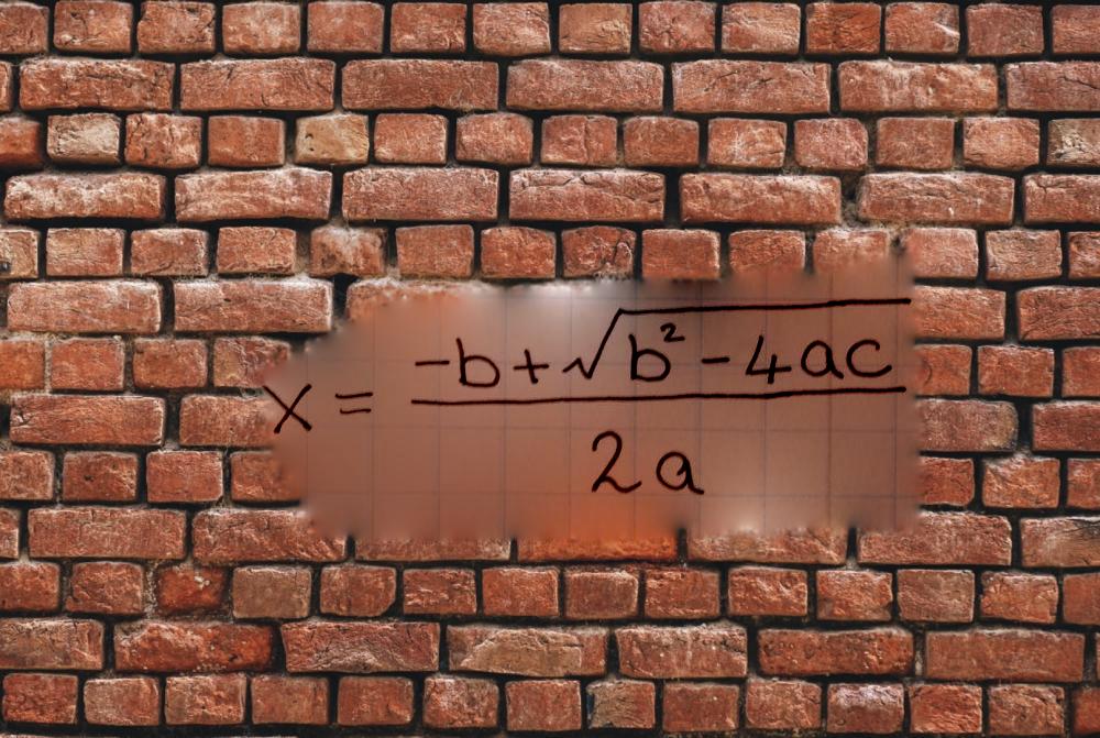
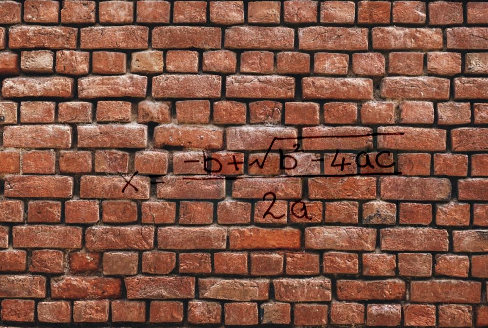
As you can see, mixed gradients will not introduce blurry parts due to the white background and will keep the features of the wall.