Gradient Domain Fusion

Part 1: Toy Problem

For the toy problem, I created a sparse matrix A. If s is the source image, and v is the image to solve for, then each row in A contains the coefficients for each pixel value in v to solve for. b is a vector of the gradient values in s. The three objectives for this problem are minimize ( v(x+1,y)-v(x,y) - (s(x+1,y)-s(x,y)) )^2, minimize ( v(x,y+1)-v(x,y) - (s(x,y+1)-s(x,y)) )^2, and minimize (v(1,1)-s(1,1))^2. For the first objective, in a row of A, the coefficient of v(x+1,y) is 1, and the coefficient of v(x,y) is -1. The corresponding value in b is s(x+1,y)-s(x,y). For the second objective, in a row of A, the coefficient of v(x,y+1) is 1, and the coefficient of v(x,y) is -1. The corresponding value in b is s(x,y+1)-s(x,y). For the third objective, in a row of A, the coefficient of v(1,1) is 1, and the corresponding value in b is s(1,1). After creating A and b, I solved for v using least squares.

Part 2: Poisson Blending

For Poisson blending, my implementations of A and b were very similar for what I did in the toy problem. But now the blending constraints to solve for are:

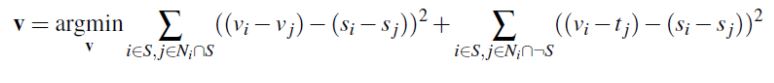
Where s is a region in the source image, t is the target image that s will be blended into, and v is the blended image. j is the 4 neighbors (left, right, up, down) of i. In a row of A, the coefficient of v_i is 1, and the coefficient of v_j is -1. The corresponding value in b is s_i-s_j. If pixel j is not in s, then the coefficient of v_j is 0, and the corresponding value in b is t_j.

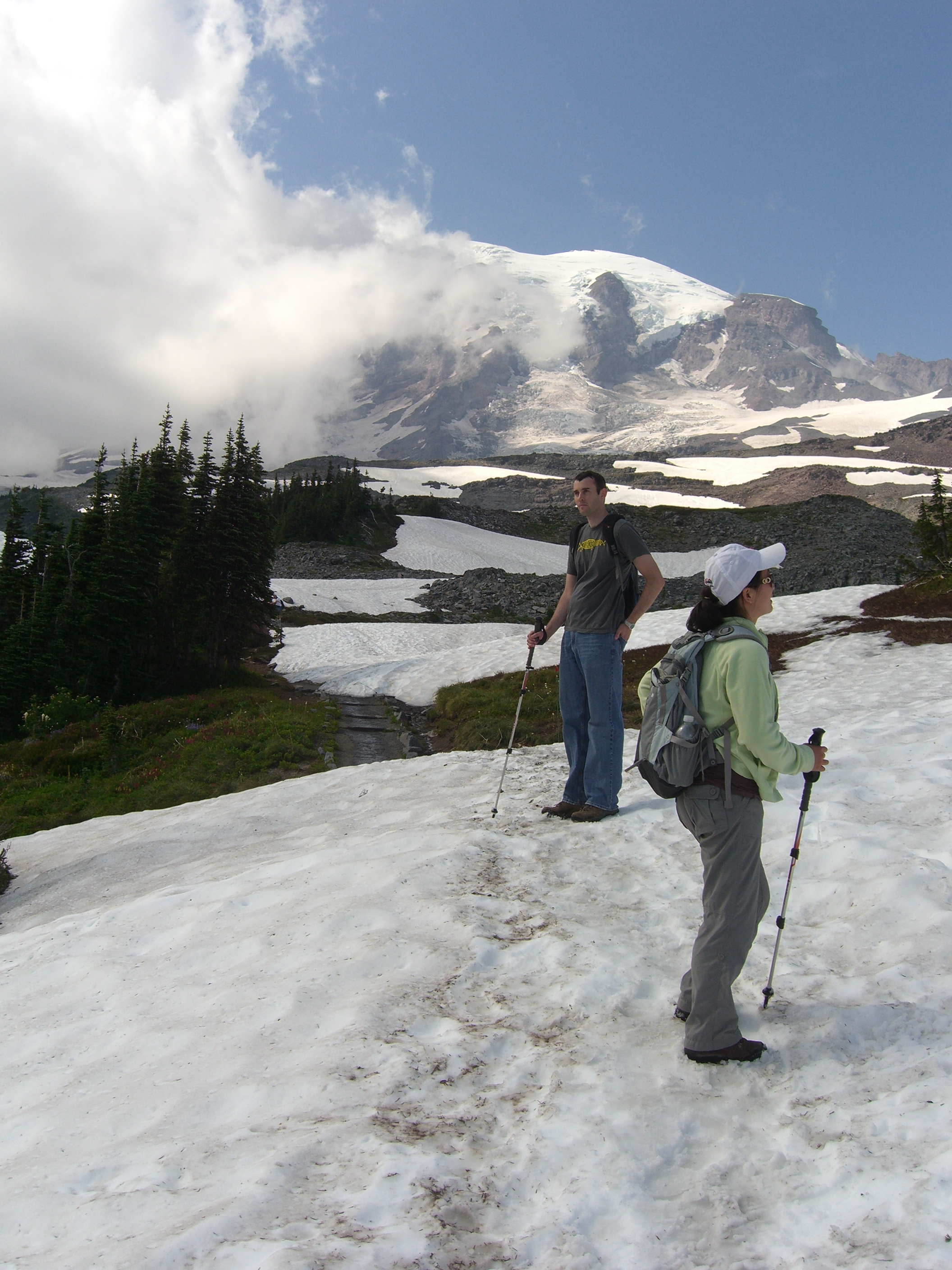
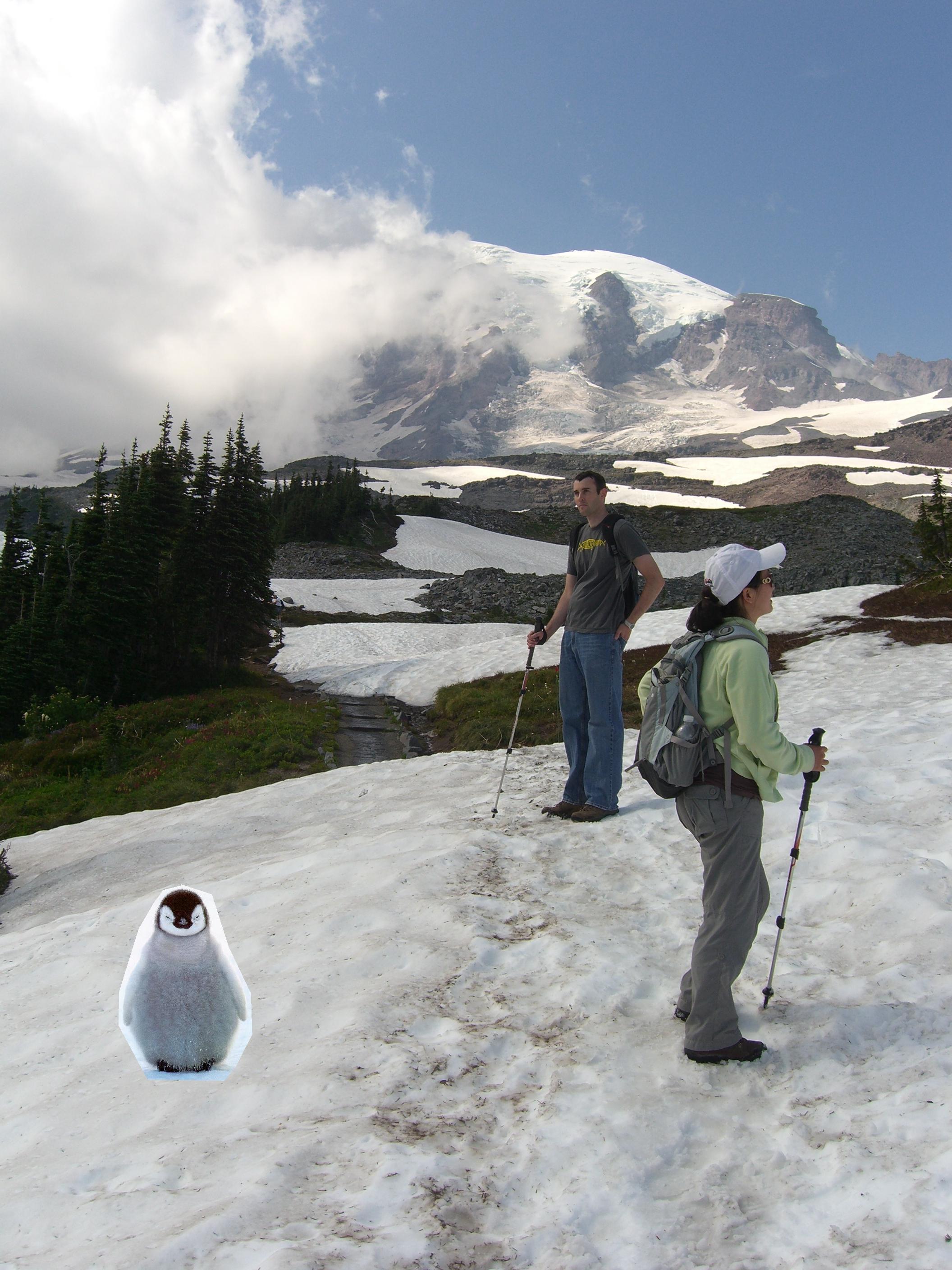
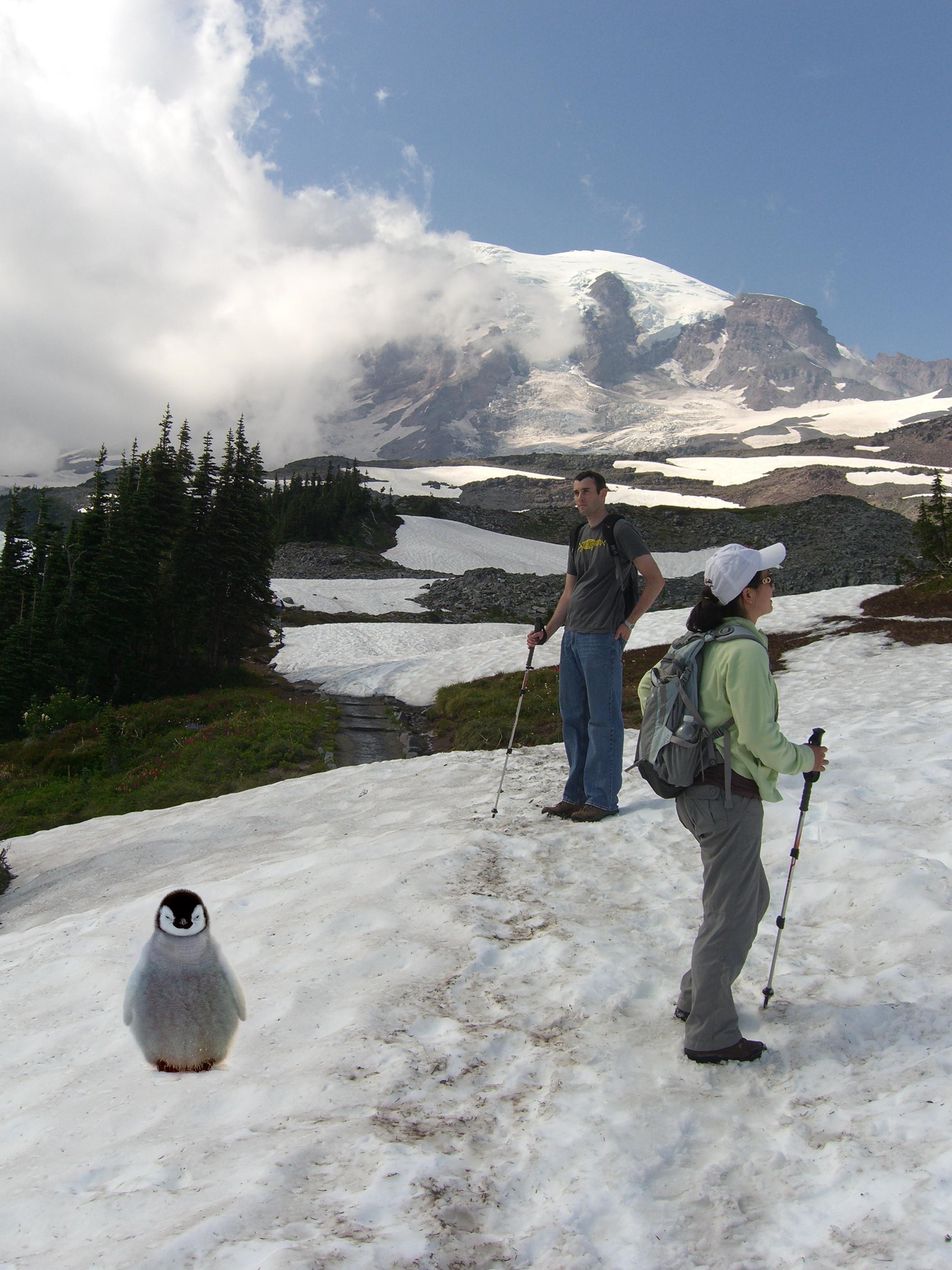
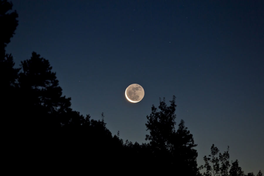
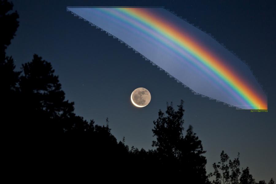
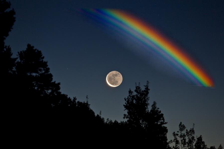
Here are my results for Poisson blending:

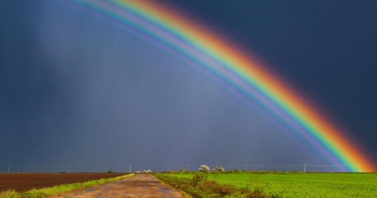
I did have one failure case when I tried to blend the rainbow image above with an image of a galaxy sky. The blending didn't look very good, most likely due to the galaxy sky having a lot of variation in colors of shades of blues and purples while the rainbow image didn't. I unfortunately did not save these images. Other than that, I didn't really have any failure cases.

Bells and Whistles

Mixed Gradients

For mixed gradients, I followed the same steps as Poisson blending but for the values in the b vector, they were s_i-s_j is abs(s_i-s_j) > abs(t_i-t_j) else they were t_i-t_j.

Final Project 2: Light Field Camera

For this project, I used the chess rectified images dataset from the Stanford Light Field Archive. There are 289 images on a 17x17 grid. The file name of each image contains the u, v coordinates of the center of projection of the camera.

Part 1: Depth Refocusing

For depth refocusing, I first found the u, v coordinates of the center image at grid position (8, 8). Then for all other images, I took their u, v coordinates and subtracted the center image u, v coordinates from them to obtain u - center_u and v - center_v. I then multiplied these differences by a constant alpha to obtain shift values that will be used to shift each image. I first tried using sp.ndimage.shift with interpolation to shift float values, but the computation time was too long. So instead, I rounded my shift values and opted to use np.roll. My results still seem prety decent despite using integers for shift values. After shifting each image (except the center image), I averaged all the images together to refocus the depth.

I varied alpha from -0.5 to 0.5 in increments of 0.1. In my implementation, a smaller, negative alpha focuses towards the back while a larger, positive alpha focuses towards the fron of the image.

Part 2: Aperture Adjustment

For aperture adjustment, I set an integer variable radius that is supposed to represent a radius of an aperture. A radius of 0 indicates the only image to be used is the center image. A radius of 1 includes the center image and the eight images surrounding the center image. As radius increases, I continue to add the images surrounding those from the prior radius.

This gif starts at radius = 0 (infinite depth of field) and increases to radius = 8 (small depth of field). At radius = 8, the silver chess pieces at the top right corner are the objects that are mainly in focus.

Part 3: Summary

In this project, I learned that by capturing light field data, I can refocus the depth and adjust the aperture, using only images. I'm amazed that I can do these things with a dataset of fewer than 300 images as I thought it would be more difficult.