Project 1: Lightfield Camera
This project was inspired by this paper by Ng et al. which shows the possible effects one can generate using a plenoptic camera.
From Ng et al., 2005: "The goal of the camera presented in this paper is to re-capture this lost information: to measure not just a 2D photograph of the total amount of light at each point on the photosensor, but rather the full 4D light field measuring the amount of light traveling along each ray that intersects the sensor."
I used data from a plenoptic camera to generate images that are focused at different depths and correspond to different apertures. The data was taken from The Stanford Light Field Archive, which contains a series of datasets: each one comprised of a set of images focused on a single subject, taken over a 2D grid.
Part 1
Depth Refocusing
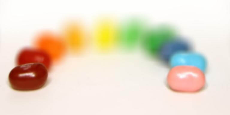
When taking multiple images of the same subject from different positions, the position of the subject will vary across the images. It is important to recognize, however, that objects placed closer to the camera will vary in position more than those that are farther away. We use this fact and calculate the average of all the images in our dataset. This will produce an image that is blurrier for objects that are closer to the camera and sharper (more focused) on objects that are farther away. Here are some sample images I generated by simply averaging all the images in each dataset.

|
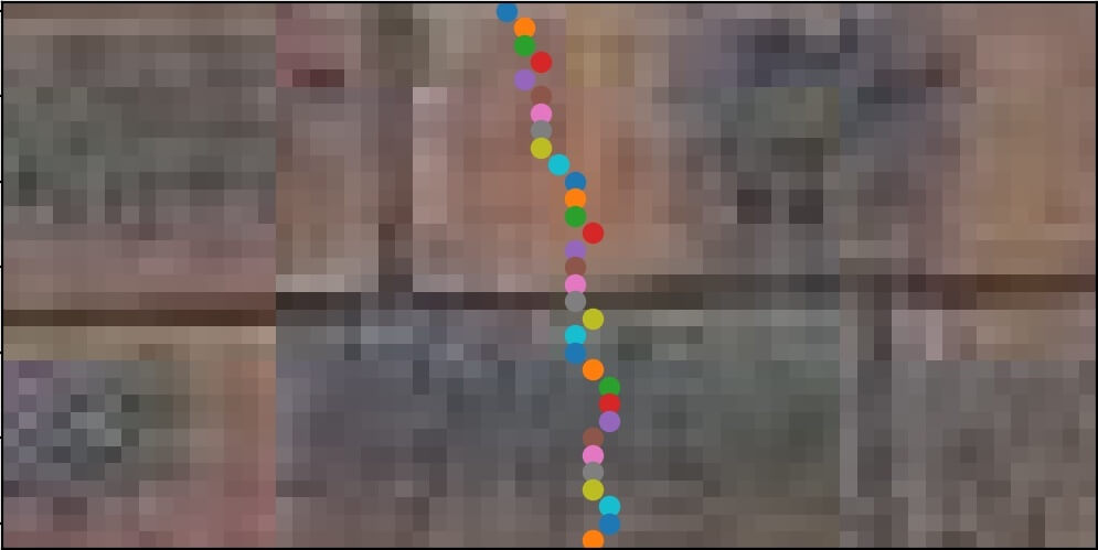
I expanded on this idea to generate images that are focused on objects in the images based on their distance from the camera. I chose one image from the dataset to align all the others to: I chose the image that is focused on the center of the image. I shifted all other images up/down/left/right based on their distance from the chosen image, times some constant, α.
In other words, for every image I in the dataset:
- Compute the vertical and horizontal distances (dy, dx) from I to Ic, where Ic is a chosen image in the dataset.
- Shift I by α(dy, dx).
The value of α will affect the depth at which the image is focused. I found that smaller/negative values for alpha led to objects that were further from the camera to be more in-focus, whereas larger/positive values for alpha led to objects closer to the camera to be in focus.

|

|
Part 2
Aperture Adjustment
Aperture in photography affects the "depth of field", or the range of depth in an image at which objects within that range remain in focus. Taking the average of many images sampled over a 2D grid (like in our datasets) will mimic a camera with a larger aperture. Taking the average of a smaller set of images will mimic a camera with a smaller aperture. To generate images that mimic varying apertures, I took a series of images with varying set sizes and computed the average image over these sets. I found that the more images I included in my averaging calculations, the more my images looked like images taken with a camera with a larger aperture. I determined the size of my sets based on the distance from each image to the center image Ic. The smallest set contained just Ic, then Ic and images that were one unit away from it, and so on.

|

|

|

|

|

|

|

|
|

|
I enjoyed this project - it was fun to see how I could use simple techniques, like averaging and translating images, to create these effects. In the future I want to try doing this to a scenee of a cityscape or photo taken from an airplane, and adjust the aperture to make it look like a miniature scene!
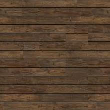
Project 2: Image Quilting
In this project I implemented the image quilting algorithm described in this paper by Efros and Freeman, "Image Quilting for Texture Synthesis and Transfer".
As described from the project spec: "Texture synthesis is the creation of a larger texture image from a small sample. Texture transfer is giving an object the appearance of having the same texture as a sample while preserving its basic shape."
I implemented both of these techniques, starting with texture synthesis. Once I had a technique for texture synthesis, I was able to use it as a base to apply my texture transfer algorithm.
Part 1
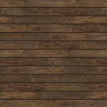
Texture Synthesis
The main idea behind texture synthesis is to sample small patches of an input texture, and choose adjacent patches that are share similar overlapping regions to create a seamless texture. To do this, I implemented three different approaches.
The first approach was to randomly sample textures. I chose a patch size and output size for my desired output texture image, and randomly sampled patches from my input texture, placing them down in row-column order. This approach led to very choppy and un-cohesive resulting textures.
The second approach was to choose patches based on the similarity between overlapping regions in the current patch and those already chosen for the output texture image. I started out by sampling a random patch from my source texture, and placing it in the top-left corner of my output texture image. Then, for every following patch, I calculated the SSD between the current patch and its neighboring patch(es) that were already in the output texture image, over a region determined by a set overlap size. In order to allow for some randomness, I chose the current patch at random among the set of all patches that had an SSD in the overlapping region with previous patches that was less than a certain value: ((Min. SSD out of all possible patches)*(1 + tolerance)). For patches in the top row, I calculated the similarity between each patch's overlapping region with the patch to its left. For patches in the first column, I calculated the similarity between each patch's overlapping region with the patch above it. For all other patches, I took into account the patch's neighbors both from above and to the left.
The third approach was very similar to the second, except instead of just placing each chosen patch down into the output texture image, I found the minimum cut between patches in their overlapping regions in order to create a more seamless transition between patches. I used the code taken from the project spec, which provided a function cut(err_patch) that takes in the error patch between two overlapping regions (i.e. for overlapping regions B1 and B2, err_patch = (B1 - B2)**2) and outputs the minimum-cost cut between them.
Here is an example of finding the minimum-cost seam between two adjacent patches.

|

|

|
|
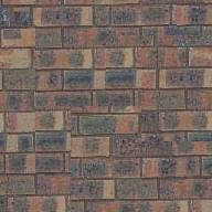
I will now display some of my results.

|
|

|

|

|

|

|

|

|

|

|
|

|
|
|
I found that my results varied a bit in their accuracy depending on the chosen patch size and output size.
Part 2
Texture Transfer
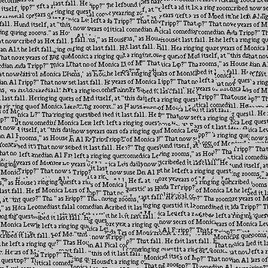
Once I had my texture synthesis algorithm, with a few minor adjustments I was able to create a function that creates a texture sample based on a secondary input image. To do this, I simply changed my cost function in choosing each patch to have an additional cost term determined by the intensity of light between the current patch and that of the patch at the target location in the second image.

|

|
|

|
|
|
Thank you for a great semester!