|
|
For the first pre-canned project I implemented, I chose the Light Field Camera. In this project, sets of images taken over the same orthogonal plane are shifted by their displacements and averaged together to produce virtual effects for both focusing at a specified depth and adjusting the aperture of the camera taking the image (which is not physically happening).
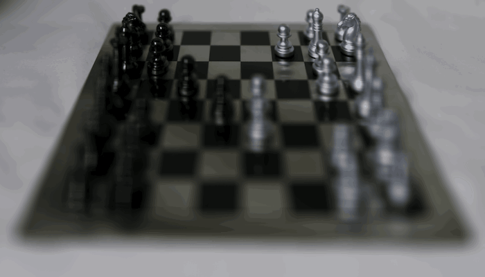
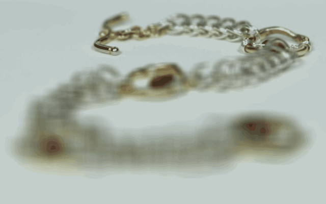
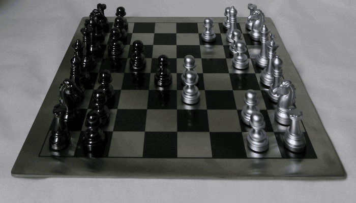
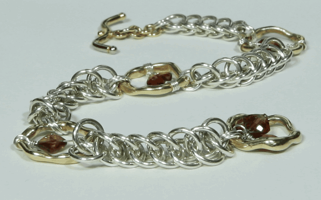
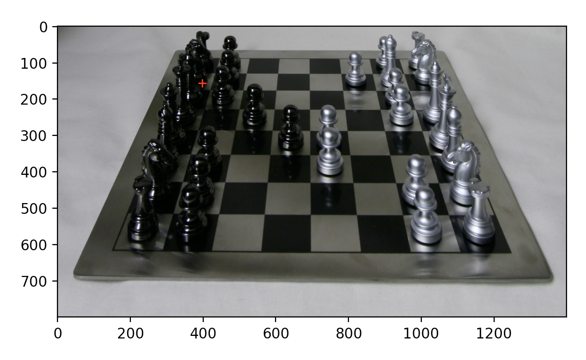
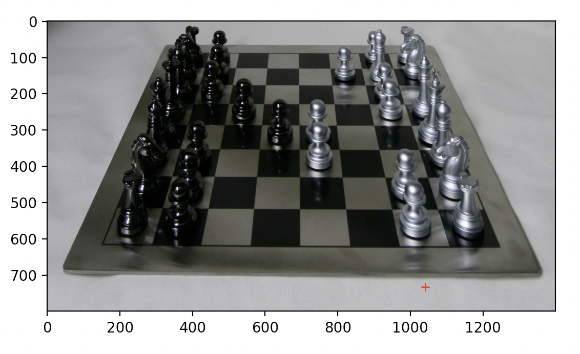
In order to virtually create the effect of depth refocusing, the set of images are averaged together. However, simply averaging the images without any shifts will cause the depth refocusing to focus on the farmost objects in the scene, as they shift only slightly in the image with each shift of the camera. To instead focus on a closer depth, the images are shifted by their displacment from a specified image. Fully shifting each image will focus on the most close objects, while instead choosing a value in between 0 and 1 and multiplying the full shift amount by that before shifting will allow for focusing somewhere in between the foreground and background. The first image set that I chose was of the chess set in the Stanford Light Field Archive, and I found that shifting by a multiple between [0, 0.75] produces good results. The second image set that I chose was of the necklace in the same archive, and I found that the best multiple range was [0, 0.65]. Below are gifs showing the refocus across these ranges:
|
|
|
To implement aperture adjustment, a center image must first be defined. Following this, the image is averaged with the shifted image of all surrounding images within a defined radius. By increasing or decreasing the radius, the aperture is adjusted. A larger radius corresponds with a larger aperture, while a smaller radius corresponds with a smaller one. Below are gifs of both the chess and necklace sets with the radius being adjusted within each frame to show how the aperture is changing. I fixed my shift multiplier at 0.3 here, which I found gave the best results when choosing the center (8, 8) image as the center of the aperture.
|
|
To implement interactive refocusing, I allowed the user to select a single point to focus on within the image. Following this, I use the distance of said point from the top to determine the depth of the point in the image. Using this distance, I then choose a shifting multiplier in between 0 and 0.75, the maximum value I determined for the chess set that would produce a clear image in the foreground. Following this, I then perform depth refocusing at the calculated depth. Below are three pairs of images, the first of which shows the point that I selected, and the second of which shows the corresponding depth refocus:
|
|
|
|

|

|
I thought it was very interesting that averaging all of these images without any shifting whatsoever would produce clear sections in the background and blurry ones in the foreground, but after reading the paper and the spec it makes much more sense. The camera itself is shifting on an orthogonal plane, which causes any shifts for background objects to appear much smaller than foreground objects. As such, averaging causes a blur for the foreground objects, but since the background ones are barely moving they still look quite clear. It is only when appropriately shifting do the foreground objects not move by much, and become more clear.
For the second pre-canned project I implemented, I chose the Augmented Reality project. In this project, I took a box and drew easily identifiable tracking points. The program would then track the points through the video, determining their locations in each frame so that a 3D box could be projected onto the 2D images.
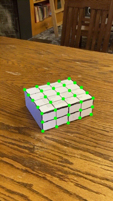
Before implementing the project, I first had to create and film the video that the 3D box would be projected onto. I chose a white box that I then used a marker to label in a gridlike fashion. The intersection of these grid lines corresponds with a single tracking point, with the bottom left point of the box corresponding to the (0, 0, 0) coordinate. The x-axis of the 3D world corresponds with the right-to-left axis of the box, the z-axis corresponds with the down-to-up axis of the box, and the y-axis corresponds with the front-to-back axis of the box. Below is the initial video that I chose. Below is a gif of the image that I chose:

|
To track points in the image, I used the out-of-the-box implementation of the CSRT tracker provided by OpenCV. This function operates over each frame and updates to find the next location of the point it is tracking within a bounding box. By repeating this for each tracker on each point, all points are tracked through the entirety of the video. Below are the highlighted points that were tracked by the tracker:
|
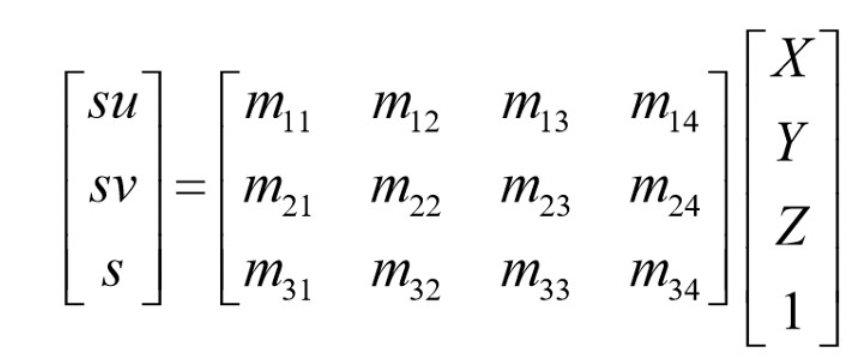
After the previous step, each frame of the video will now have a set of corresponding 2D image points. Since each point has a corresponding 3D world point, a homography matrix is computed using least squares to find a way of warping an object in 3D space to the 2D image. Below is the formula that was used, which was taken from lecture:
|
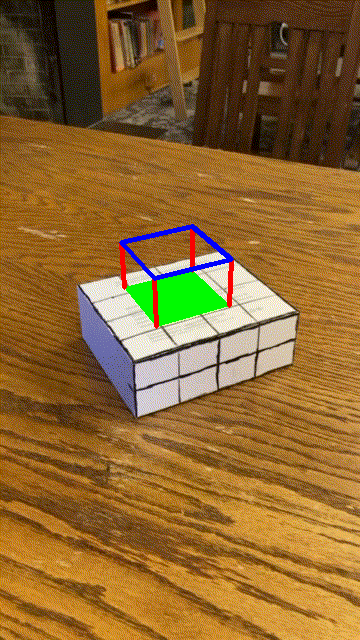
Once a homoggraphy matrix has been computed for each individual frame, a 3D box is defined at the corners (1.5, 1.5, 2.5), (1.5, 4.5, 2.5), (4.5, 4.5, 2.5), (4.5, 1.5, 2.5), (1.5, 1.5, 4.5), (1.5, 4.5, 4.5), (4.5, 4.5, 4.5), and (4.5, 1.5, 4.5). These corners place the box at the top of the white box I used to track movement in the scene. For each frame, the homography is used to warp these 3D points onto the 2D image space, and the draw function then draws the 3D box so that it appears as if inside the scene. By doing this for each individual frame, the entire output can be composed into a gif. Below is the comparison between the input video and the output video with the 3D box:
|
|
|
This was certainly my favorite project of the two, as I found the use of the tracker to be very interesting. Becasue the tracker could be used to extrapolate tracking points for each frame, there was no need to compute a method of transferring the 3D box coordinates between the frames. Rather, the implementation computed a warp for the box to each image so that it looked correct for that specific image, then put together all of the images into a cohesive video.