Project 3: HDR Imaging

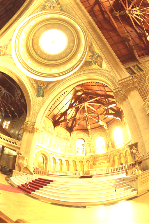
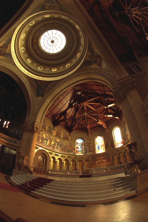
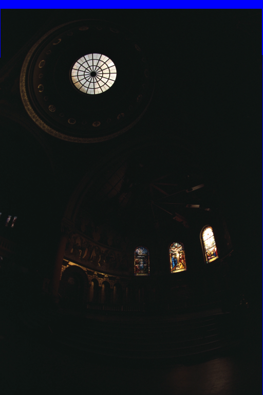
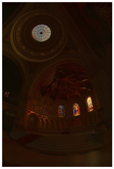
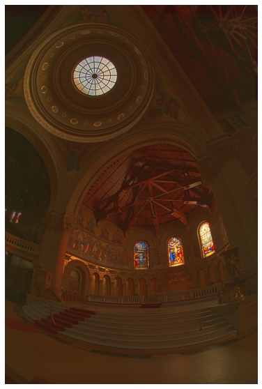
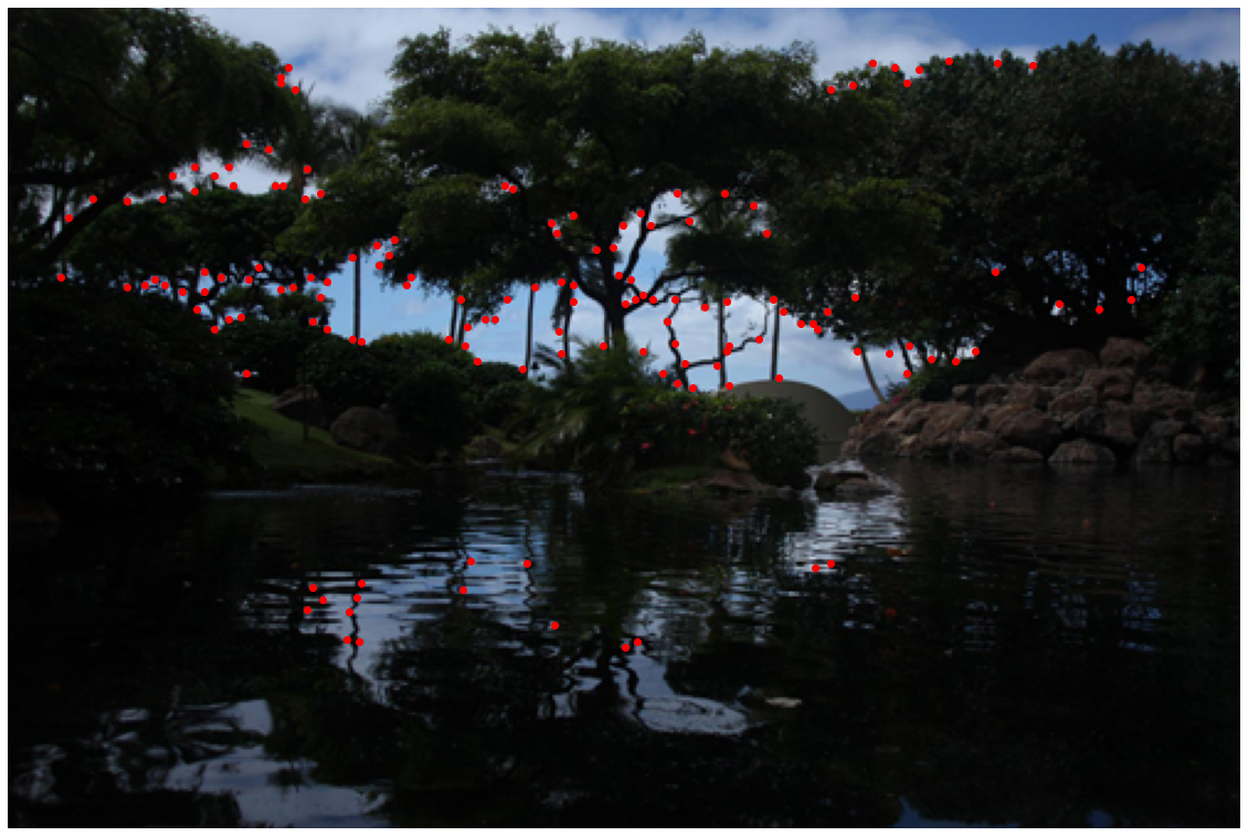
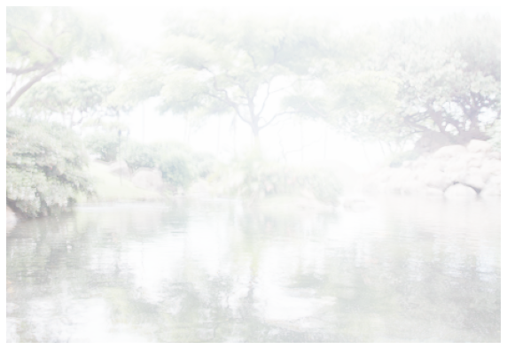
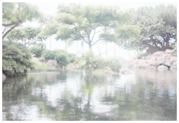
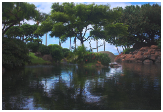
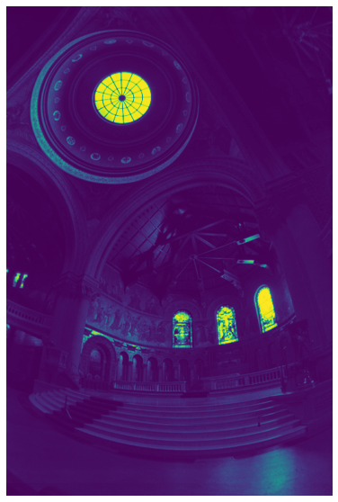
We want to build an HDR radiance map from several LDR exposures. Essentially, given several exposures of the same scene, we wish to recover the original radiance of the scene.

Variables:

1. E is the scene radiance at pixel i.
2. Zij is the observed pixel value for pixel i in image j, and is some function of that pixel’s exposure. f(Ei Δtj)
3. Ei Δ tj is the exposure at a given pixel in a given image. It is the scene radiance multiplied over some time interval
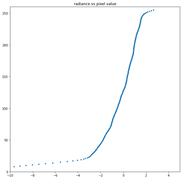
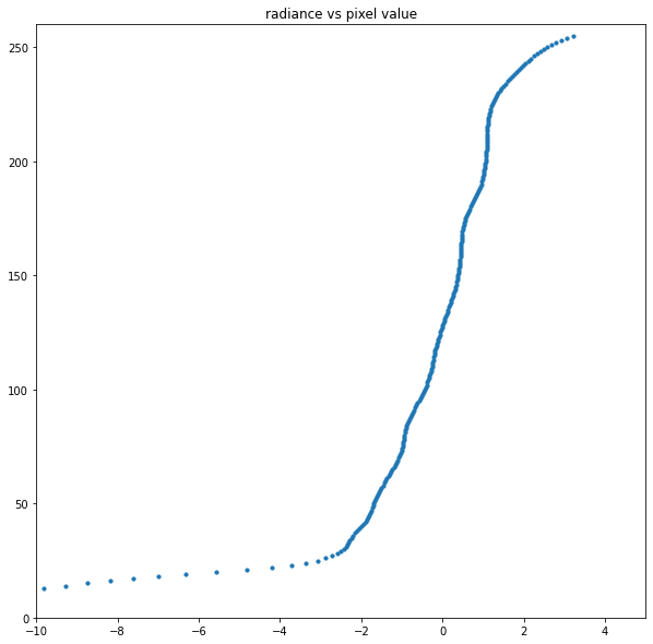
4. f is some sort of pixel response curve. Instead, we solve for g = ln(f-1), which maps from pixel values (0 to 255) to log exposure values
5. g(Zij) = ln(Ei) + ln(tj)

The key here is that Ei remains the same across each image.

Finding g sounds extremely difficult, but it becomes much easier when you consider the constraint that its domain is simply the possible range of pixel brightness values (256); thus, its range is also finite.

Thus, g is simply a mapping of 256 input values to 256 outputs, and can be modeled as a least-squares approximation problem.

We also introduce a few other effects on our optimization:

• We constrain that g(Zmid) = 0, where Zmid = ½(Zmin + Zmax). We arbitrarily assume that the pixel value of middle brightness has unit exposure.
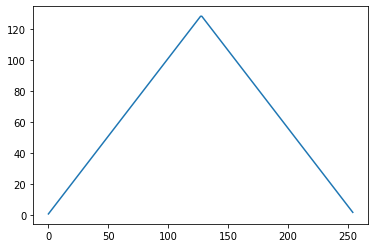
• We introduce a weighting function w(z) with a triangle curve in order to less punish jagged curves near extremes and induce the function to optimize for smoothness near the middle of the curve. Our images will naturally have discontinuities, thanks to noise affecting darker parts of the images and clipping affecting the brighter parts.
  

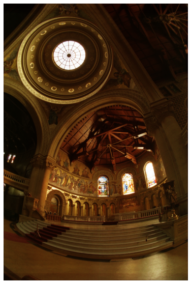
Having solved our optimization problem, we now have g(). We may recover pixel radiance via this formula. 

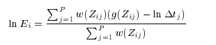
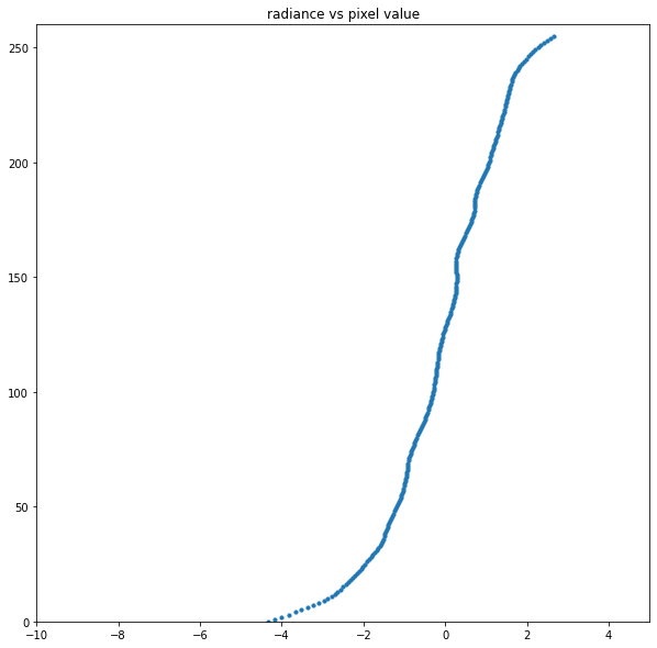
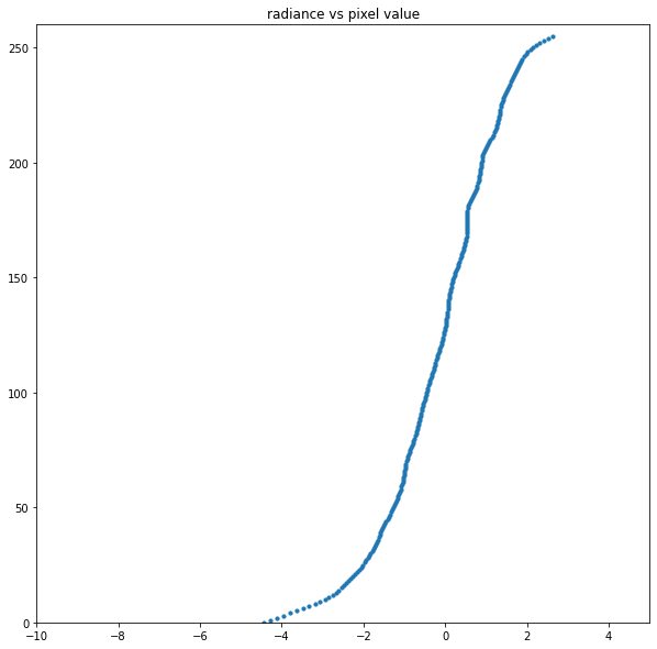
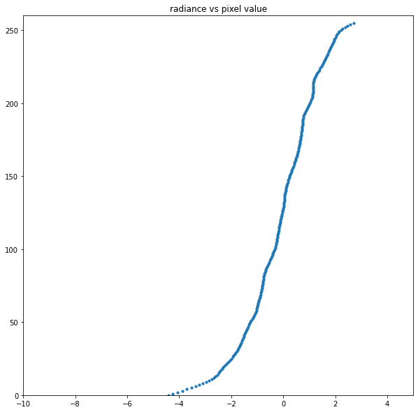
Here are the radiances and response curves for red, green and blue, respectively.

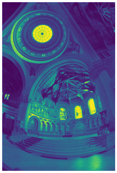
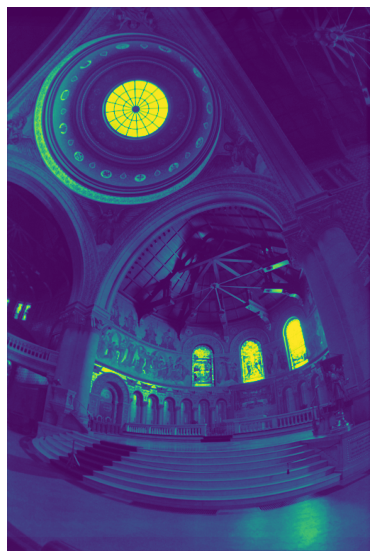
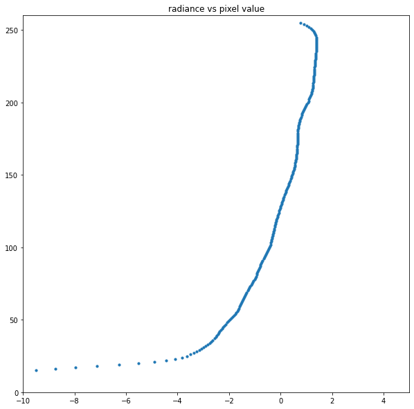
There is some nonlinearity in the response curve at the highest blue values. I would put that down to the relative unavailability of data points with such high blue values. Thankfully, this and the fact that the nonlinearity only kicks in at around B=249 also means that this nonlinearity of the response curve shouldn't have a huge aesthetic effect on the final image.

Now, in order to display the image we need a tonemap function to map these radiances to pixel values.

I started by implementing a simple global tonemap operator f(x)=x/(c+x)

This function has the benefit of having a tunable parameter. c is a positive number; the lower its magnitude, the more overexposed the image becomes as the x/x term dominates and the function converges towards f(x)=1

My image was initially a bit underexposed, so I applied my operator at c=0.6.

The result is very nice! However, we are still losing a bit of detail on the brightest (stained glass windows) and darkest (wood beams on the ceiling) parts of the image.

The solution is local tone mapping. Durand and Dorsey outline an approach that separates the image data into three different channels: base, detail and color.

First, we derive the intensities (averaging radiance for each channel) and chrominances (the ratio of a channel's chrominance to the intensity per pixel). These are our 'color' layer.

We isolate a 'detail' layer by denoising via a bilateral filter to find the 'base' layer, and subtracting the filtered image from the original. (we perform these operations on the log intensities, rather than the original image)

We then rescale and offset our base layer to ensure that its maximum intensity is 1 and that to ensure that it has 5 stops of dynamic range.

We then recombine with the detail layer to reconstruct the log intensity, and then multiply by chrominance to reconstruct our color channels.

Very nice! Much more detail is visible, and the colors look great with a bit of scaling (red and green were multiplied by a factor of 0.9). All that's left now is to perform a little bit of post-processing to adjust the exposure.

it's gorgeous. I love it so much.

The Brown projects offered extra credit to implement automatic image alignment.

For this step, I chose the garden exposure stack from the brown website. There is some movement of the camera during the photos, so the merged stack from the website looks blurry.

In order to align the images, I adapted my project 4 implementation, which used Harris corner detection, ANMS local point suppression and RANSAC to estimate the homographies between the garden images.

I aligned every image to image 4 in the stack. I suspected that the middle image would contain a good mix of points present in both the most and least-exposed images.

After aligning the images and cropping out the edges, I put the images through my code from parts one and two.

Along the way, I also made some accidental art when displaying the radiances. The sky is so bright that this scene looks like a moonlight night.

Anyway, here are the response curves of R, G and B for the garden photos. As you can see, the curve is much better behaved this time.

I tried applying the global tonemap function with c=10,50,100,200,400 and 800. The image is much more well-lit this time, so these c values that are orders of magnitude higher need to be applied. However, the results look quite unsaturated. We can do better than this :)

Here it is with local tone mapping and a bit of post-processing. It does look a little oversaturated, but I'm happy with my results. The trees look so vibrant!