CS194-26 Final Project

Rishi Upadhyay, rishi.upadhyay@berkeley.edu, 3033975663

Light Field Camera

In this project, we used existing light field datasets to generate visualizations of changing focus and aperture. We did this by taking images that were taken at slightly different positions and re-aligning them before averaging. By varying the amount of position correction, we were able to adjust the depth of focus, and by adjusting how many images we included we were able to adjust the effective aperture. The project is split into two parts, depth of focus and aperture:

Depth Refocusing

To achieve depth refocusing, we adjusted how much position correct we applied to every image. This is because by default, with no correction at all, the back of images will be in focus since those objects move very little even as the camera moves. On the contrary, the objects in the front will be out of focus. Therefore, if we apply the perfect correction, we should ideally have an image that is perfectly in focus in the front but out of focus in the back. Therefore, in this part, we found the range of correction values that gave us images focused in the back to images focused in the front and then created a montage. In practice, this was done by finding the offset from one image to another and then scaling it by a constant, a hyperparameter of the system. A constant of 0 is no correction. Here is this montage:

Aperture Adjustment

In this part, we adjusted the effective aperture of the image while keeping the depth of focus constant. We achieved this by observing that averaging together multiple images that are spread out over space is the equivalent to having a larger aperture. Therefore, for this part, we started with just one image and then added images based on distance from the original image. This allowed us to slowly add further and further images, thereby allowing us to increase our effective aperture as we went along. To choose the depth at which these images were focused, I looked at my results from the last part and chose the hyperparameters that allowed me to focus the image on the middle. Here is the montage of aperture changing:

Bells & Whistles: Using Real Data

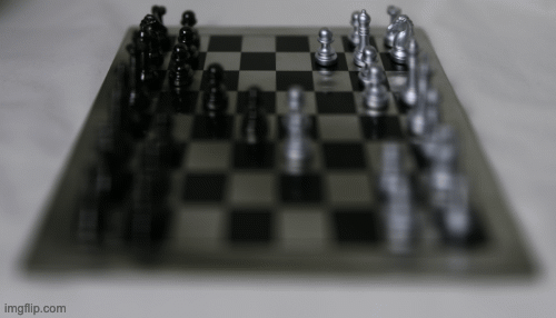
I also implemented a bell & whistle for this project. I chose to try to use real data that I collected to create a light field. To do this, I took a grid of images of items on my desk with my phone. I kept track of the movement between each picture and then added that information into the system like we did for the given data. I then ran both depth refocusing and aperture adjustment. Here are all the images overlayed with no correction:

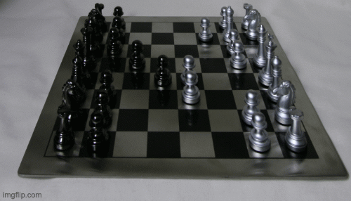
Here is the depth refocusing:

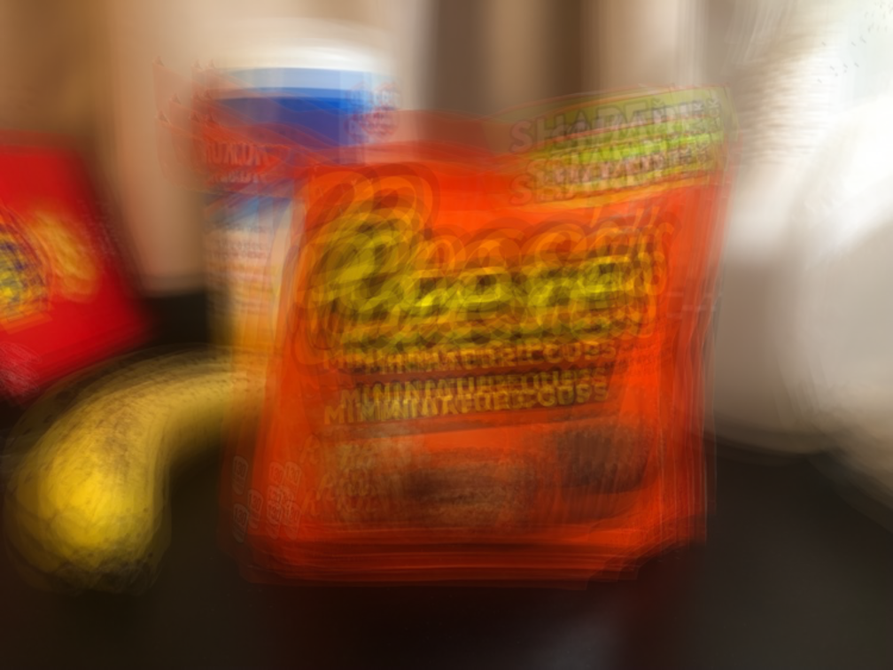
Here is aperture adjustment:

Clearly, these results are poor. I believe this is mainly because the data collected was not very precise. Despite my best efforts, I was not able to make sure that the translation between images was accurate because of difficulty in measuring and making sure the camera didn't move. In addition, I did not have as many images as the given datasets, so the system has less data. Having a better way to capture the images would greatly improve this.

Gradient Domain Fusion

In this project, we use gradient domain fusion to add a source image into a larger target image with smooth boundaries. The goal was to create smooth combinations without sharp boundaries or other artifacts. In order to do this, we used image gradients. Essentially, we imposed a few constraints on our pixels in the area where we wanted to add our source image (we will call this the modification area). Each pixel had 4 total constraints, with two different types of constraints: 1. Source Image to Source Image: this was when a pixels neighbor was also in the modification area. The constraint here is that the difference between the two pixels in the new image should be as close to the difference in the original picture as possible. 2. Source Image to Target Image: this was when a pixels neighbor was not in the modification area, i.e. was in the background. In this case, we enforced the constraint that the difference between these two pixels in the new image should be as close to the difference of the two pixels in the target image as possible. For each pixel, we check all 4 neighbors and apply constraints based on the type of neighbor. The constraints are represented by a linear system of equations in matrix form. We then find the least squares solution to this system to get our output image. Here are some outputs of this system:

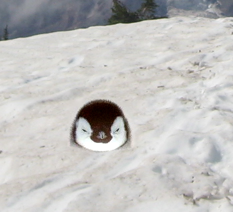
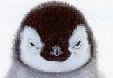
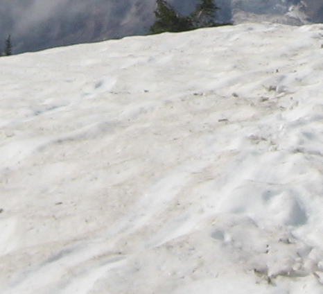
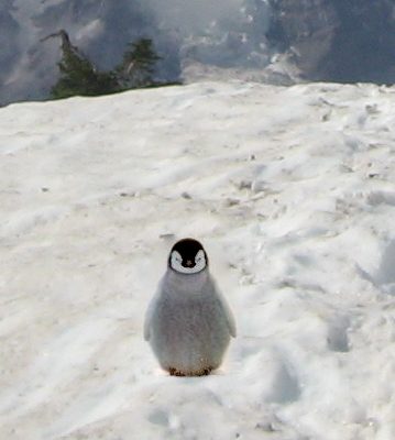
This is the head of the penguin combined with the ice. Here are the original images:

Here is the penguin example but zoomed in for the sake of processing time:

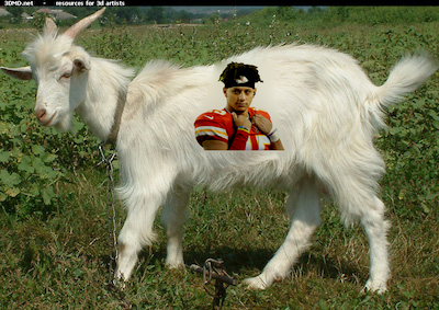
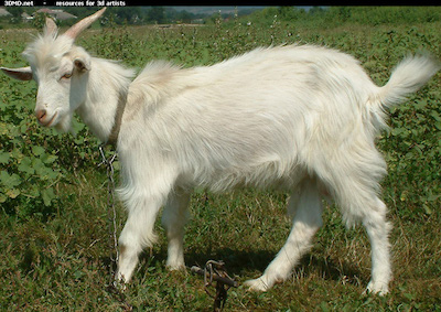
For this example, the original two images are also shown:

There is also a failure case, likely because the colors did not match up: