In this project, we will achieve complex results such as depth refocusing and aperture adjustment through the shifting, averaging, and manipulation of lightfield data.
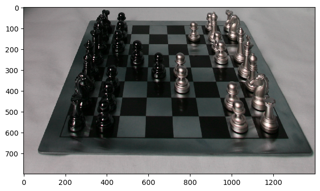
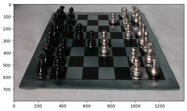
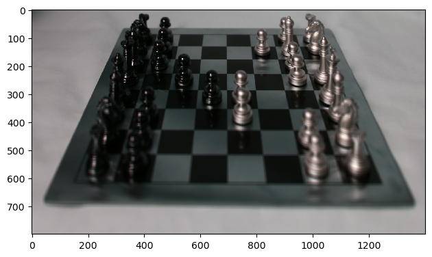
This project wouldn't have been possible without the lightfield images and information provided in the Stanford Lightfield Archive. In particular, I chose to use the images of the chessboard from the archive.
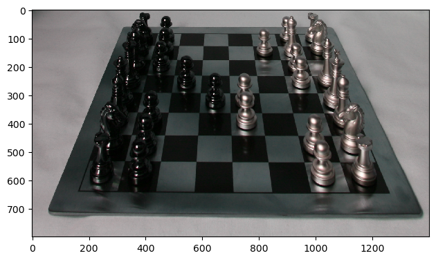
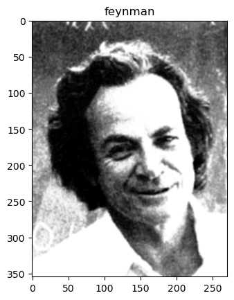
Below are 2 out of the 290 images of the chessboard from the dataset, specifically the 1st and 201st images. You can see slight differences in the position of the chessboard relative to the camera / viewer.
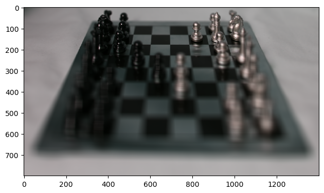
The first thing I did was compute the average chessboard image given the images of the chessboard from the dataset. I did this simply by averaging each color channel (R, G, B) of the dataset images separately and then combining these average channels into a singular image. Below, we can observe that the objects nearby in our field of view tend to see more blurring / motion compared to further away regions which appear sharper; this is because nearby objects on average see greater shifts with changes in our camera position relative to further away objects.
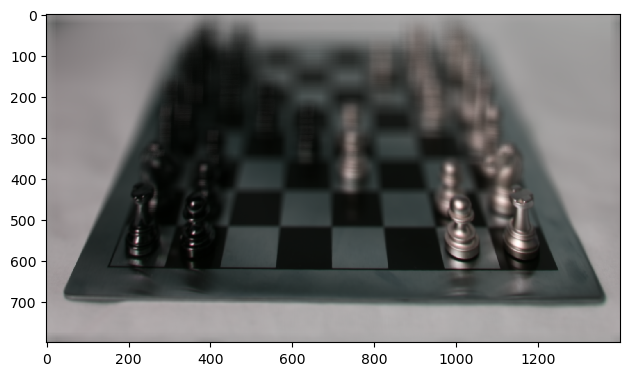
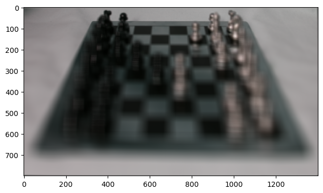
In this part, I "shifted" the images in the dataset so as to construct averages (using all the images) which would focus at different depths. To do this, I first computed the average u,v coordinates of all the chessboard images in the dataset. Then, I subtracted this average from each image's u,v coordinates; scaled this result by a variable, alpha, based on where I wanted the focus to be positioned; and translated each image based on these scaled u,v coordinates. The results are shown below.


This GIF is composed of cross fading the above depth refocusing images.
In the final part of this project, I averaged differently set sizes of images in order to mimic cameras of varying aperture. In particular, I expected to see that averaging a large number of images would mimic a camera with high aperture whereas averaging a small number of images would mimic a camera with low aperture. In order to do this, I fixed the alpha for the depth adjustment to a particular value (e.g. 0.1) and restricted the images I used to compute the average to those that fell within a certain range / field of the mean u,v coordinates. The larger / more permissive I made the range, the more I saw high aperture camera-like results, and the smaller / more restrictive I made the range, the more I saw low aperture camera-like results.
Below, the dimensions of the grid correspond to the range within the mean u,v coordinates I had set for images to be counted towards the resultingly computed average.


This GIF is composed of cross fading the above aperture adjustment images.

I'm still deeply fascinated / rocked by the sheer number of effects you can simulate given a bunch of images and their light field data! This was my favorite project in the class :)
In this project, I implemented image quilting algorithms which enabled applications such as texture synthesis (making a larger texture image from small samples) and texture transfer (giving an object the same texture as a sample while maintaining its shape).
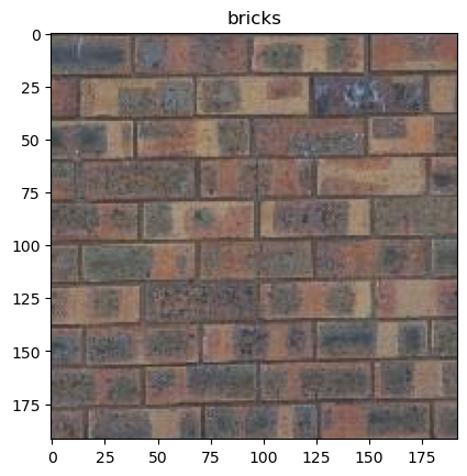
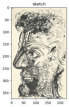
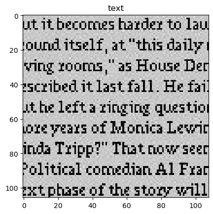
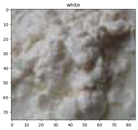
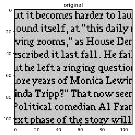
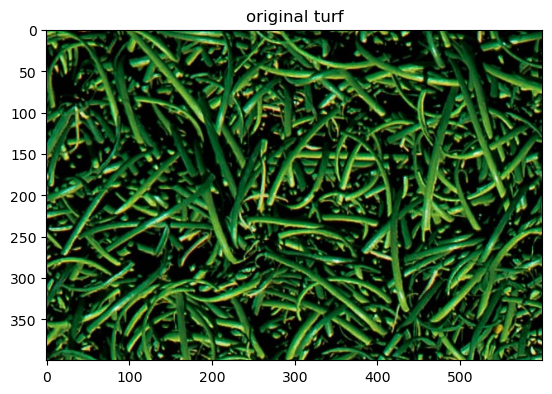
The following textures are all ones I used for this project; I found them here.
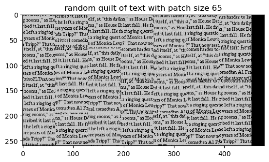
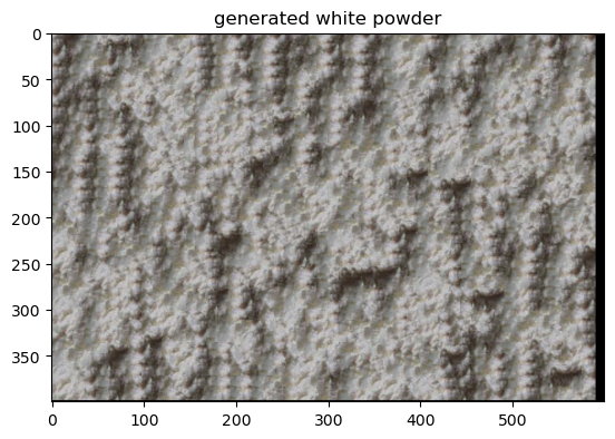
The first quilting algorithm I implemented was one that randomly sampled square patches of a particular size from a sample in order to synthesize a larger output image (image synthesis). I implemented this simply by randomly sampling patches from the sample texture and placing them adjacently to one another. We can see from the result below that the random patch based approach isn't very successful at building smooth, convincing larger textures.
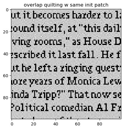
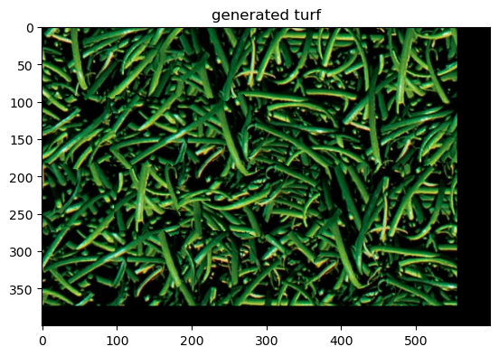
In this part, I made the original quilting algorithm a bit "smarter" by analyzing the edges / overlaps of our patches, computing a cost function, and only admitting patches into the quilt which fell under a certain cost threshold. This approach, simple / overlap quilting, led to slightly more successful results.
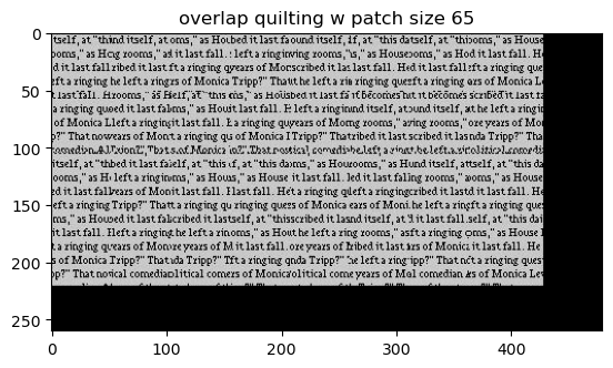
While my quilt_simple function worked rather well at making the visual patch flow smoother, there were still several edge artifacts which were contributing to cutoff words and incoherency in the current result. I improved on this in the next part.
In this part of the project, I added a function to help me find the min-cost contiguous path across patches to improve the quilt_simple algorithm. I did this by implementing / adapting a dynamic programming cut algorithm (inspiration cut.m file here) that would help me find this contiguous lowest cost path and also compute the seams / masks indicating the pixels I would need to transfer over to my result.


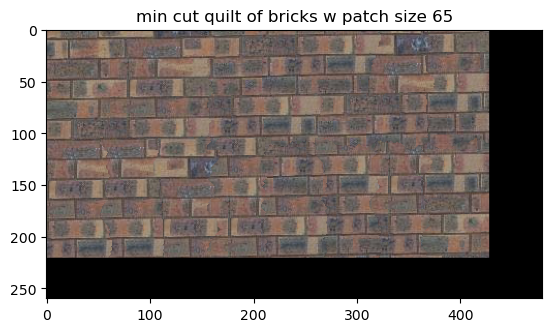
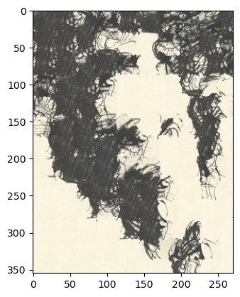
I also visualized the min cost path (as asked in the spec) by highlighting the overlapping images and their cut mask.
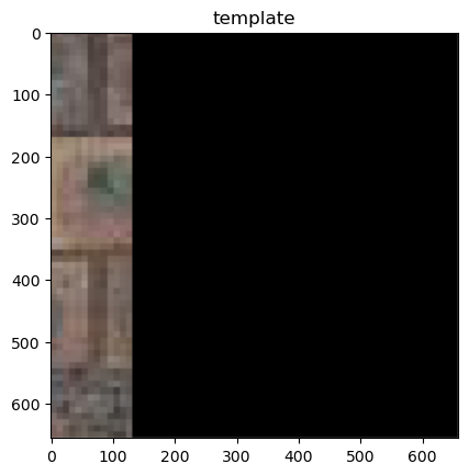
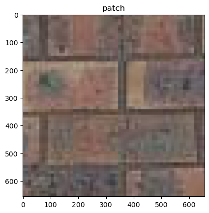
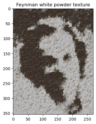
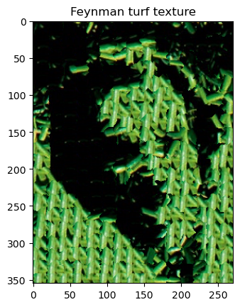
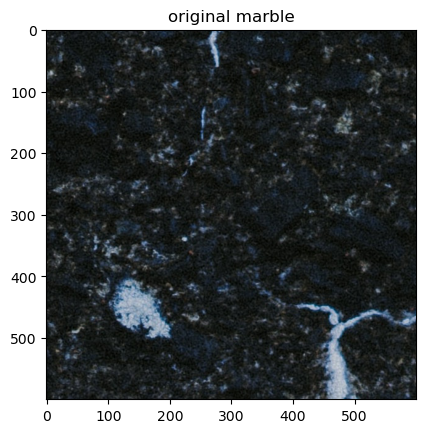
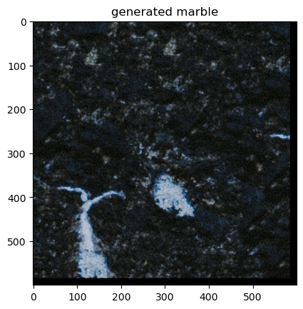
Finally, in this part I implemented texture transfer (giving an object the texture of something else), which was essentially the same as my quilt_cut function with the addition of a cost term between the sampled source patch and target patch.