The rays of sunlight both illuminate and energize our environment. In relation to photography, every outdoor photo is sharply influenced by the sun’s relative position. How much information can we infer about the relative position of the sun when considering an image, time, and location? This work explores the current status of image-based time prediction via solar azimuths.
A main source of inspiration is prior work from Efros that tries to calibrate cameras given a sequence of images from webcams distributed throughout the US . The majority of the algorithms that the paper introduces seek to specify the camera parameters (focal length fc, zenith θc, and azimuth ϕc). The work also introduces an algorithm that performs camera location estimation using clear sky images, the sun’s position, the date, and the local time. Even though the bulk of the algorithm that the authors introduced in that paper, they were impressively able to achieve a mean error of 110km on real low-resolution, Internet webcam streams.
Since the publication of this prior work, the average cell phone camera quality has increased dramatically. This change in quality (along with cell phones’ increased societal normalization) means many more images which have a few key impacts on this research space. Images that are taken with a cell phone often feature precise geographical information, as this information is already needed for providing cell service. Additionally, image capture time is much likelier to be accurate for similar reasons, especially when compared to traditional DLSR/mirror-less cameras.
In addition to cell phones yielding higher-quality images with higher quality metadata, there are now more publicly available images. Websites such as Flickr and Instagram serve as a nexus for photo takers to share their images, creating a wealth of possible training data. Flickr especially is amenable to this growing set of images, with a policy that lets users upload as many images as they like for free. Even conservative estimates put the annual set of captured images at over 1 trillion .
Time is a natural and naive first choice to use as a proxy for solar illumination. This makes sense, since human inference can easily make a temporal prediction when going outside. However, there are several drawbacks that make time non-viable in many cases. First, latitude directly influences solar lighting. The sun rises and sets at different times based on how close you are to the equator. As a result, simply stating the local time is not sufficient to infer how the environment will be illuminated. Second, the current date also directly influences solar lighting. The current date’s relative position to the solstice or equinox drastically changes the sunset and sunrise times. As a result, we simply cannot use the time to describe the illumination properties of an image captured outdoors.
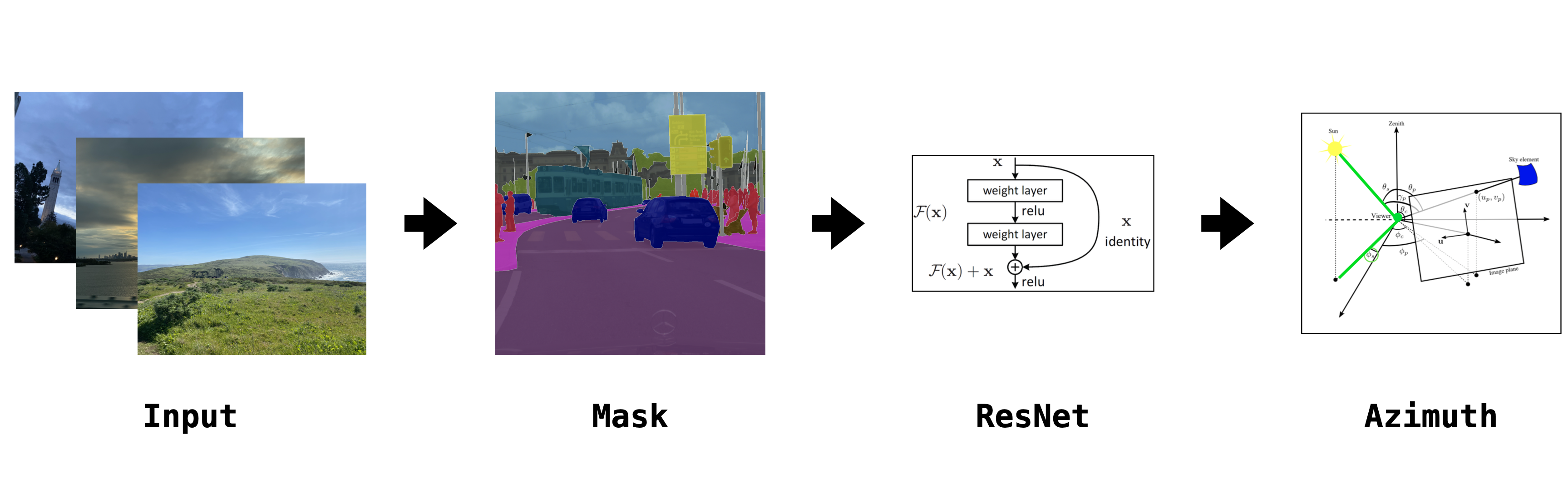
Instead, this project uses the solar azimuth (e.g., the sun’s height in the sky). This angle is akin to how close the sun is to being directly overhead. There is also a convenient relation between solar time and azimuth angle, provided you know other relevant image metadata. In this equation, ϕs is the solar azimuth angle, θs is the solar zenith angle, h is the hour angle, in the local solar time and δ is the current sun declination or sun position.
A novel related method for computing the solar azimuth from subsolar points was published as recently as this year, which could be an even more accurate and useful translation between azimuth and local time .
The circular nature of the sun's revolution means that disambiguation between cases with similar lighting conditions (e.g., sunrise vs sunset) is difficult. To circumvent this issue, I flatten the circular path of the sun’s image across the sky to a single line. Conceptually, this means that the model will only be returning how near or far you are from noon or midnight—not an exact time. However, this limitation means that modeling the azimuth is more amenable to loss criteria like mean square error, relative to a point on a circle. An alternative method could be to use discrete classes for classification (e.g., night and day) but this is far less impressive of a result.
Another limitation of this solar azimuth method is that it still does not address different weathering patterns, and is likely going to be prone to some noise for high variance weather locations. San Francisco is one popular example of how drastically the weather (and with it the solar illumination) can vary in a short amount of time. However, any other method which does not directly consider weather patterns present at the time of image capture will also suffer.
There were several promising datasets that I considered using for this task. An initial exploration led me to the Yahoo Flickr Creative Commons 100 Million Data- set (YFCC100M) data set . This dataset holds nearly 100 million images sourced from users on Yahoo and Flickr under the creative commons license. A dataset of this size would be very powerful, but also even more challenging to train than other available datasets. Additionally, YFCC100M was pulled from Yahoo’s dataset library Webscope at the time of writing (Dec. 2021).
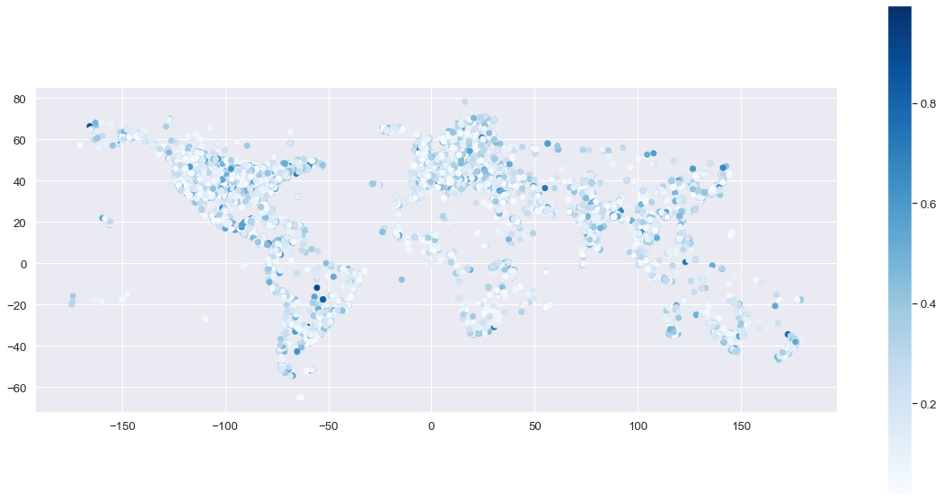
Further exploration led me to another dataset with 14 million geographically distributed images . Geography is much more important for this solar azimuth prediction task than tag/object/class inclusion. The sun’s movement is more tied to physical location than specific objects or activities to recognize. Due to the nature of the prediction task, having a broader set of physical locations in your database is advantageous. One interesting crawling technique the authors employed when creating this was to use the social graph of Flickr to more robustly explore physical space. They also filter the images based on the accuracy level of the reported geographical location, setting the loosest acceptable precision to city-level.
While I explored this dataset, I realized that a majority of images were simply not going to be usable for various reasons. Note that even since the time of this dataset’s publication (2014), cell phone cameras have come very far for low-light image capture. Many images contained only indoor scenes or were very close-up pictures. Other pictures suffered from poor lighting or illegibility. The expressive training power of the larger dataset was also turning out to be hindered by poor example images.
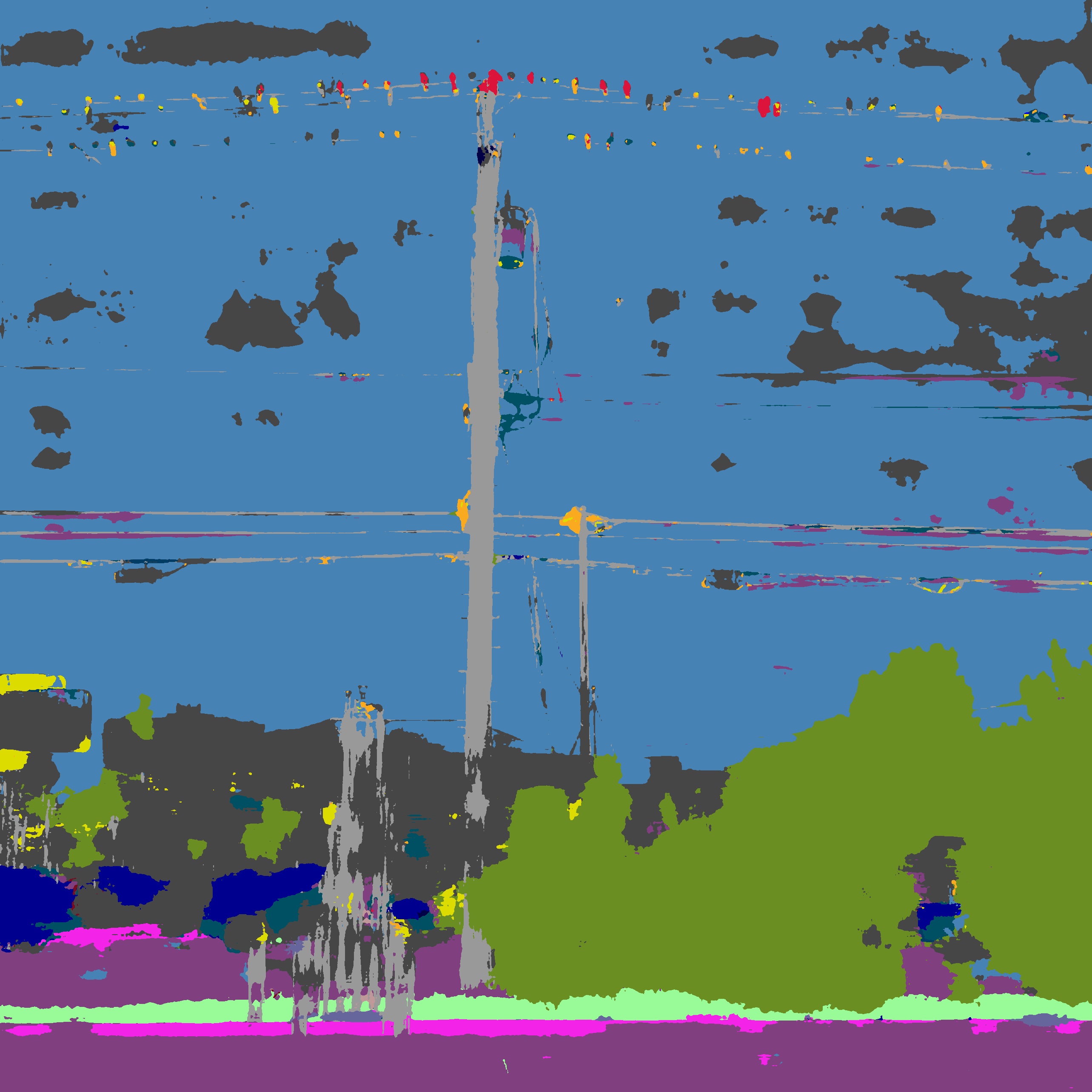
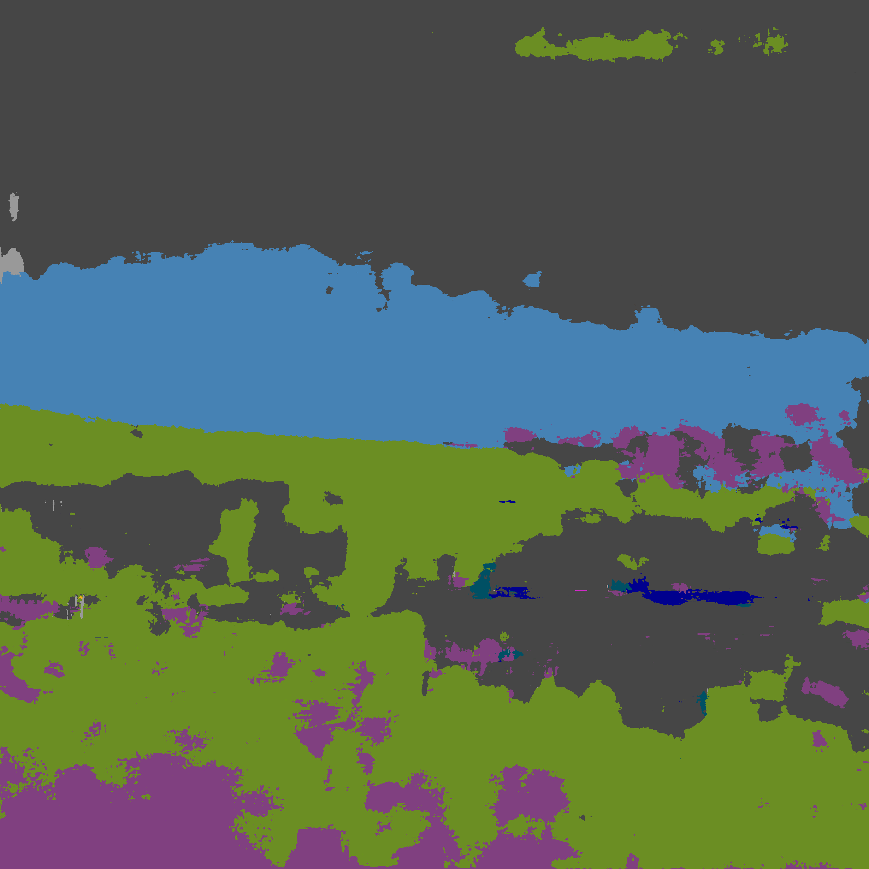
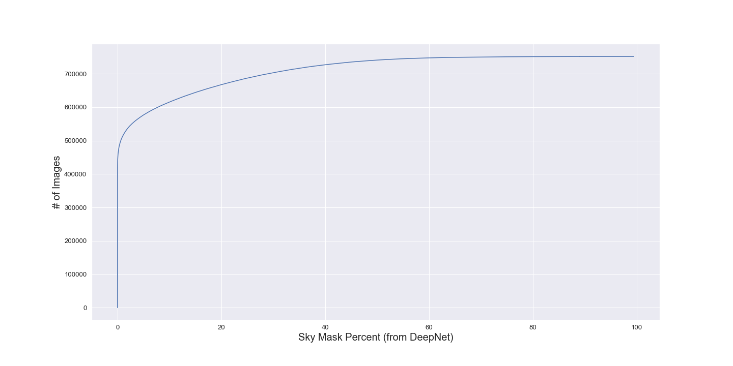
To solve this issue, I use a network that can detect whether the sky is present in an image. This technique leverages DeepLab , which is used to segment an image into one of 19 different class labels. The key aspect of this class set is that it includes a ’sky’ label, which can be used to further filter images. DeepLab segments the dataset images, and we save the semantically-labeled image mask. For this project, I used a pre-trained version of DeepLabV3+ to segment the training images. This model was pre-trained on the Cityscapes dataset . From this mask, we can simply count the pixels that correspond to the sky label. To normalize for image size, we record the percentage of pixels associated with the sky. This serves as a convenient mechanism for filtering through images that are less unlikely to be useful for our training data. We are likely throwing away some decent outdoor images which could be shot from a downward angle. However, the size of the dataset is too large is currently not an issue so trimming for quality at this stage in the processing pipeline works well.

Despite the database doing a decent job at selecting information, I found that the resulting data-set post-sky-filtering had many outliers. To further ensure that the final training examples were of the highest quality, I also did several sanity checks to prune these outliers. One such technique was filtering for any image years between 1999 and 2015.
Another step to improve performance is to crop from the bottom of the image to create a square image shape. The architecture I used takes in images of (244, 244), where the default camera shape is often rectangular (and not square). To avoid image warping effects from squeezing the image into a square box, we can make an assumption about the image orientation. By assuming the sky is mainly going to be at the top of the image, we can crop the bottom and retain a higher chance of gaining useful visual cues for the azimuth. With that said, I have not run a comparative performance test to see if removing this crop dramatically affects the model’s performance.

I used a pre-trained ResNet50 model with PyTorch to try and predict the solar azimuth angle. The inputs to the network are a normalized three-channel image. The output is the estimated azimuth angle, ranging from 0. We compute the ground truth azimuth angle from the image capture month/day, latitude, and longitude, which is used for loss. However, I faced persistent issues with data loading large libraries of images on Google Colab. One strategy I was in the middle of implementing was filtering images into prefix-based folders. For example, file 123456.jpg would be sorted into a folder 12/34/123456.jpg to lower the number of files per folder. Ultimately, I was unable to create any meaningful results with this network (or others). Still, I believe that with the proper loading setup to handle this larger image dataset the model can yield strong results.
Much more effort and time went into securing and filtering the data than expected. Additionally, working with larger image sets was a stumbling block that held me back. While it is frustrating to feel limited by mundane and unrelated technological issues, I am undeterred. I really enjoyed working on this project and hope to continue my progress even beyond the class or semester.
I see several interesting directions for possible future work.
See architecture or results.
Currently, this project aims to predict the azimuth angle. This serves as a shift-invariant analog to the time of day. The complement to this is the zenith angle, akin to the time of year. A follow-up idea is to have models try to predict this angle, effectively estimating the date of the image capture.
If the performance of the solar azimuth model is sufficient, could it be used as a drop-in discriminator for GAN-based image transformation? I am interested in more precisely transforming images to realistically appear at a different time or date by leveraging this model’s performance.
My current azimuth model ignores the direction of time (e.g. sunrise vs. sunset). Theoretically, light from the sun hits the earth the same way in both cases though. Still, an interesting question: are there phenomenological traits that could be learned to distinguish between rising and falling days. People’s behavior certainly varies from morning to night, so one idea is to infer from image activities or population. As a stretch goal it could be interesting to try and predict the season (e.g. differentiating seasonal transitions).
Intuitively, humans can very easily estimate time of day simply by being outside. This project is a first step towards modeling that intuition with visual information in a neural network. I leverage a 14.1 million image set that is globally distributed sourced from Flickr. I filter images by selecting those which are composed of at least 10% sky to select outdoor images. The modeling attempt works off of a pre-trained ResNet model but fails to showcase decent results. While the current project status is limited, I think an impressive set of results is in reach in the near future.
Thanks to Professors Efros and Kanazawa along with the rest of the teaching staff for an amazing semester.
David Carrington. 2021. How many photos will be taken in 2020? https://blog.mylio.com/how-many-photos-will-be-taken-in-2020/

Liang-Chieh Chen, George Papandreou, Florian Schroff, and Hartwig Adam. 2017. Rethinking Atrous Convolution for Semantic Image Segmentation. ArXiv abs/1706.05587 (2017).

Liang-Chieh Chen, Yukun Zhu, George Papandreou, Florian Schroff, and Hartwig Adam. 2018. Encoder-Decoder with Atrous Separable Convolution for Semantic Image Segmentation. ArXiv abs/1802.02611 (2018).

Marius Cordts, Mohamed Omran, Sebastian Ramos, Timo Rehfeld, Markus Enzweiler, Rodrigo Benenson, Uwe Franke, Stefan Roth, and Bernt Schiele. 2016. The Cityscapes Dataset for Semantic Urban Scene Understanding. 2016 IEEE Conference on Computer Vision and Pattern Recognition (CVPR) (2016), 3213–3223.

Kaiming He, X. Zhang, Shaoqing Ren, and Jian Sun. 2016. Deep Residual Learning for Image Recognition. 2016 IEEE Conference on Computer Vision and Pattern Recognition (CVPR) (2016), 770–778.

Jean-François Lalonde, Srinivasa G. Narasimhan, and Alexei A. Efros. 2009. What Do the Sun and the Sky Tell Us About the Camera? International Journal of Computer Vision 88 (2009), 24–51.

Hatem Mousselly Sergieh, Daniel Watzinger, Bastian Huber, Mario Döller, Elöd Egyed-Zsigmond, and Harald Kosch. 2014. World-wide scale geotagged image dataset for automatic image annotation and reverse geotagging. In MMSys ’14.

Bart Thomee, David A. Shamma, Gerald Friedland, Benjamin Elizalde, Karl S. Ni, Douglas N. Poland, Damian Borth, and Li-Jia Li. 2016. YFCC100M: the new data in multimedia research. Commun. ACM 59 (2016), 64–73.

Taiping Zhang, Paul W. Stackhouse, Bradley D. Mark Macpherson, and J. C. Mikovitz. 2021. A solar azimuth formula that renders circumstantial treatment unnecessary without compromising mathematical rigor: Mathematical setup, application and extension of a formula based on the subsolar point and atan2 function. Renewable Energy (2021)