The idea of recovering structure from motion is not new and has been around for a few decades. However, I found epipolar geometry to be quite confusing and the idea of being able to recover 3D coordinates from 2D images by simply moving the center of projection of a camera is quite fascinating. In order to gain greater familiarity and understanding of epipolar geometry and to demystify, from my perspective, the technique of extracting 3D coordinates for detected features from 2D images taken using the same camera but different centers of projection, I decided to implement my own structure from motion solution which generates 3D point clouds from input images.
My implementation uses the following general structure. I calibrate my phone’s camera using built-in calibration tools provided by OpenCV. This step gives me the intrinsic matrix associated with my phone camera which are used in later computation to apply epipolar constraints. I then recover the pose of the camera, in world-coordinates by computing a homography matrix that rectifies a known texture within the scene. This texture is determined beforehand and is always present in the scene. These world rotation matrices and translation vectors for each image are used to compute relative poses for the camera in relation to another image. It is these relative poses which are then used to construct the essential matrix used for the epipolar constraint step. Alternatively, the texture need not be present in the scene. Since we know the intrinsic matrix of the camera, we can estimate the fundamental matrix using the 8-point algorithm. Using the camera intrinsic matrix, we can then extract the essential matrix from the fundamental matrix and decompose the essential matrix to extract the relative rotation matrix and translation vector associated with an image pair.
Epipolar constraints are applied to the keypoint matches in order to filter out most of the bad matches between image pairs. Using either the essential or fundamental matrix, if a matched keypoint in the first image does not fall on, or very close, to the epipolar line of the second image, then the match is discarded. A perfect match, a keypoint which falls on the second image’s epipolar line, would produce a value of 0 within the constraints function, but due to image noise, keep points with a certain degree of tolerance, or values less than 0.0001. Though this constraint does not remove all of the bad matches, it removes enough to generate a relatively clean 3D point cloud with few errors and using an even smaller threshold value discards too many keypoints, some of which are actually good matches.
From the filtered keypoints that pass the epipolar constraint, I proceed to recover their depth values using singular value decomposition. These depth values are then multiplied with each normalized keypoint in order to get their approximated 3D coordinate which is stored in a numpy array and displayed as a point cloud using the built-in tools of open3d. By working through the concepts behind epipolar geometry and implementing a solution to constructing 3D point clouds from 2D images, I learned a lot about the based ideas behind structure from motion and have a much better understanding of how epipolar geometry can be applied to recover 3D structures from 2D camera images, but with different centers of projection.
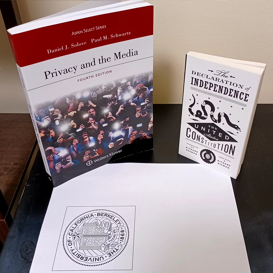
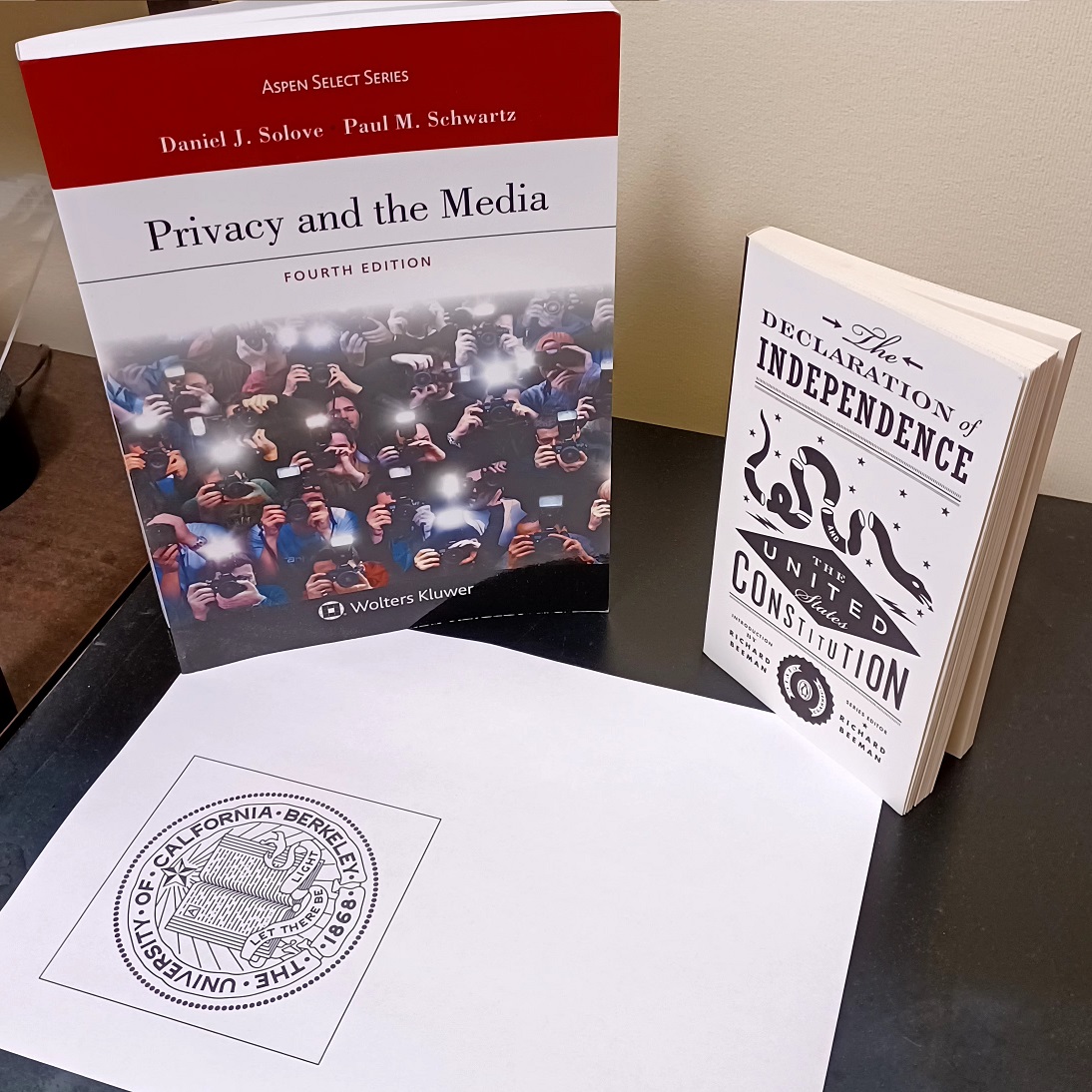
Before reconstructing the point cloud, getting images of the scene and the reference texture (if being used) is the first step in the process. Though it may seem trivial, in my testing I noticed that that 3D point cloud generation would become extremely sparse if the scene images lacked texture-rich objects. For example, an object that exhibits a relatively uniform color with an oversimplistic texture resulted in the feature detectors not being able to identify a sufficient number of unique keypoints that could be matched with another image. Consequently, the point cloud was not as detailed due to the lack of matched keypoints. To overcome this issue, I selected objects to photograph that appeared to have complicated textures, such as surfaces with a lot of text or high frequency information such as changing colors across the surface, corners, and edges. Below are two examples of scene images I took with feature texture-rich objects along with the reference texture used to recover the camera pose in world coordinates (if not using the fundamental matrix method).
In order to recover the essential matrix, either from the relative pose between two cameras or from the fundamental matrix, we have to know the intrinsic camera matrix. I recover the intrinsic camera matrix, and also account for any distortion in the images, by using OpenCV’s built-in camera calibration tools and suggested method for performing camera calibration [4]. I take about twenty pictures from different angles of the OpenCV checkerboard pattern of size 9x6 with my phone camera (which is very cheap as the phone itself is a budget smartphone). I then call the built-in function findChessboardCorners in OpenCV to detect the appropriate corners in the calibration images which are then used to call the calibrateCamera function. This function returns the camera’s intrinsic matrix and the distortion parameters along with rotation and translation information for the camera. I then recover the camera’s calibrated intrinsic matrix along with the region of interest by calling getOptimalNewCameraMatrix, another built-in OpenCV function. I can then use the calibration parameters: camera intrinsics, camera new intrinsics, and distortion to undistort each of the scene images taken by the same phone camera. I also crop the images using the region of interest parameter, also returned by the calibration method. The scene images are now undistorted and ready for processing. Especially when using a cheap camera like the one that comes with a smartphone (particularly a budget smartphone) this calibration step is crucial for generating more accurate 3D point clouds since the camera distortion produced by smartphone cameras can be quite significant.
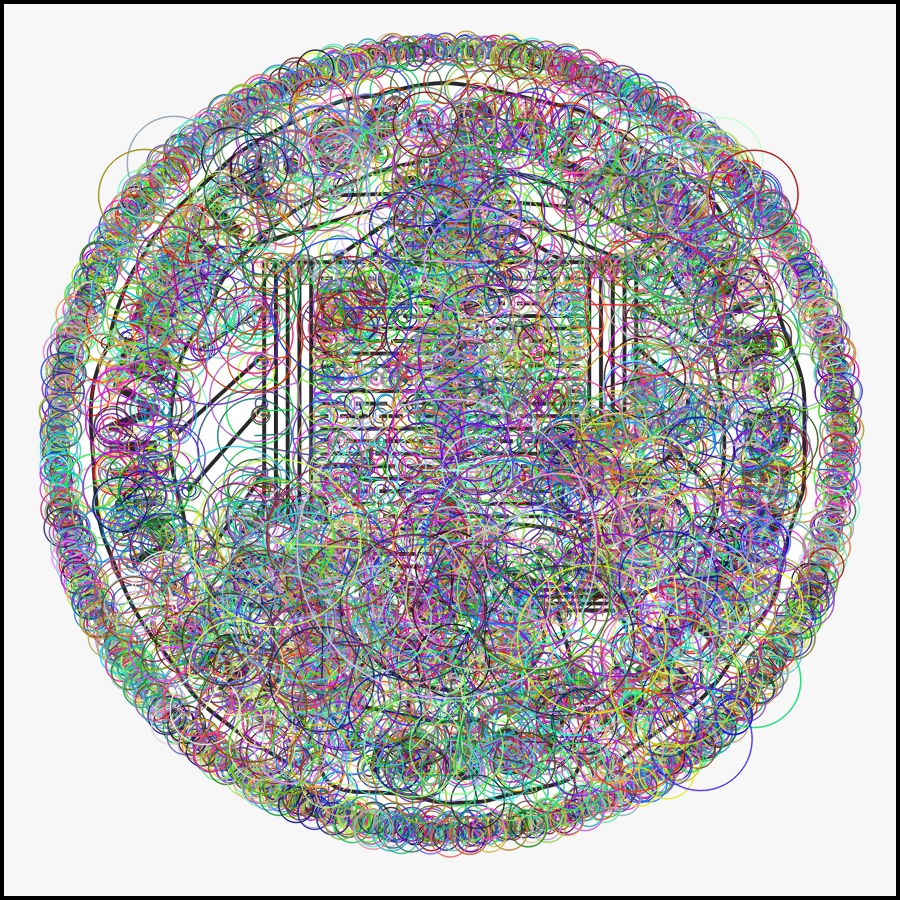
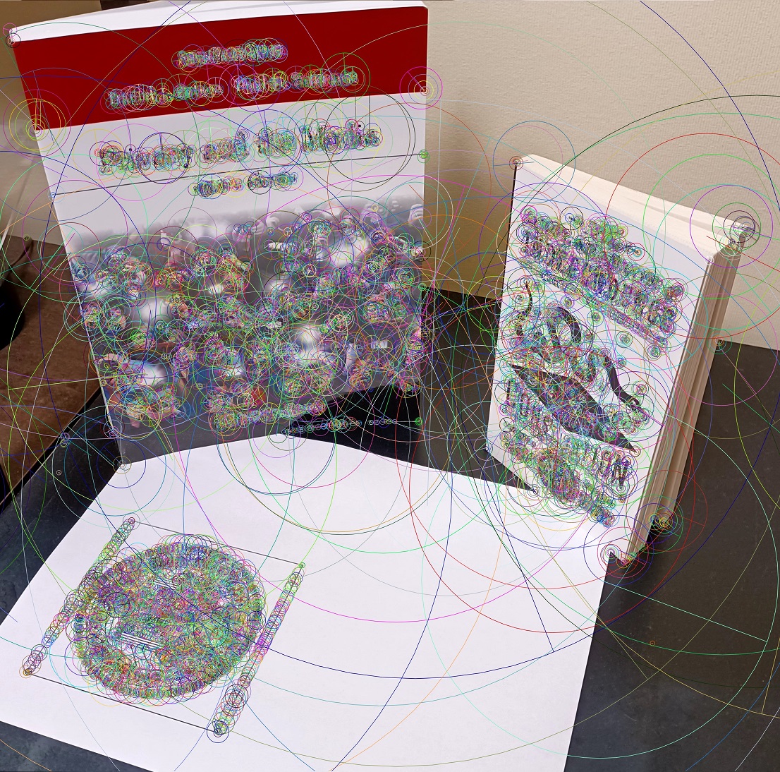
In order to perform any kind of reconstruction from 2D images, features need to be detected within each of the images and then matched to another image. I use OpenCV’s implementation of the BRISK feature detector which is both scale and orientation invariant. I settled on using BRISK over other feature detectors after reading Tareen and Saleem’s paper [5] which compared the SIFT, SURF, KAZE, AKAZE, ORB, and BRISK feature detection algorithms for performance, accuracy, and invariance to scale and rotation. Their results showed that BRISK was nearly as accurate as SIFT and also one of the most efficient feature detection algorithms. In addition to BRISK being an open-source feature detection algorithm, I decided to use the BRISK feature detector for my reconstructions. Likewise, following the recommendations in the OpenCV documentation [1], I initialized my feature matcher to a brute force matcher which used the norm hamming distance between features to detect a match. Crosscheck was also enabled to improve the accuracy of initial feature matches. Below are displayed a couple of examples of the BRISK keypoints being detected in images, with points represented the detected feature and the rings around the points representing the different scales used by the BRISK algorithm to generate a descriptor which describes the feature.
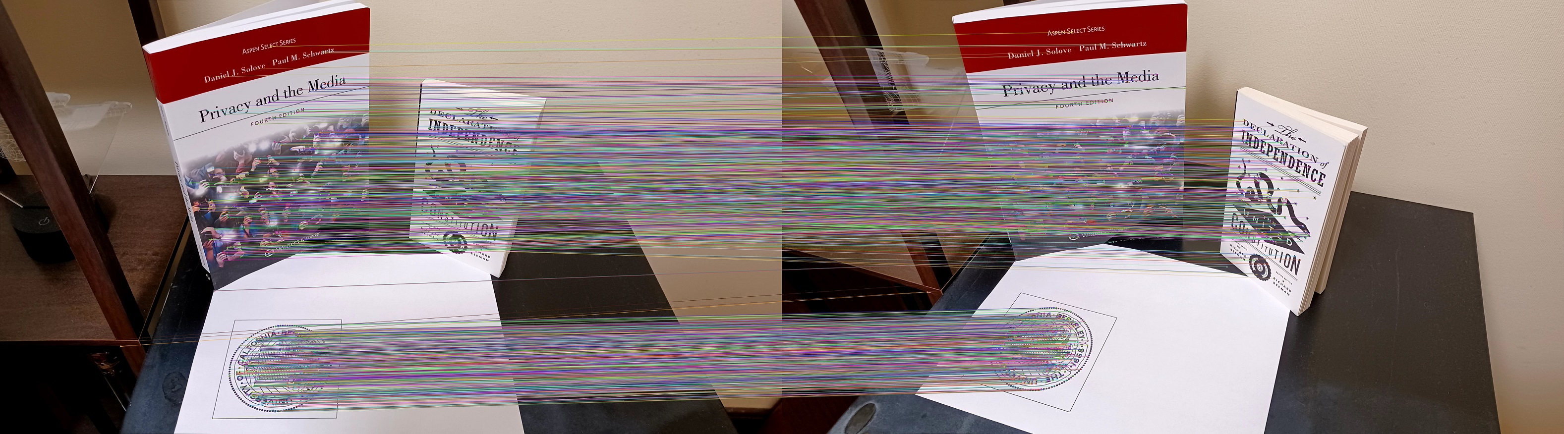
In the following steps, we can directly compute the Essential matrix used to enforce epipolar constraints from knowing the relative rotation matrix and translation vector that transforms a point in one camera to the same point in the matched camera pair. One way to recover the relative rotation matrix and translation vector is to first compute the camera pose in world coordinates for each image taken. I do this by placing a known texture in the scene for every image I take. In this case, the known texture is the UC Berkeley seal. Since I know the dimensions of the printed UC Berkeley seal, I can scale the coordinates of the detected features from the known texture image (the left image in figure 2) to fit the size of the texture in each scene as follows:

The above equation is dividing each of the keypoints by the texture’s image shape, which is square so we can just use one of the dimensions, and then multiplies it by a scaling term, in this case 0.101 since the dimensions of the printed texture were 10.1 centimeters. I then compute a homography transformation matrix which rectifies the known texture in the scene so that it matches the texture image. The homography matrix is computed using the set of keypoints between the texture image and one of the scene images. I run RANSAC in order to reduce the possibility that the computed homography is erroneous due to a bad match. This rectification encodes the world rotation and translation of the camera taking the image and can be retrieved by decomposing the computed homography. I first normalize the homography matrix by multiplying it if the inverse of the new intrinsics matrix for the camera. This puts the computed homography into normalized camera coordinates rather than image coordinates. I then follow the OpenCV documentation describing how to recover camera pose from homography [3]. In brief, I compute the product between the norms of the first and second columns of the homography and take the square root of the product. This scalar is then used to normalize all coordinates in the homography by dividing all elements in the homography by the scalar. The world translation vector is now the second column of the normalized homography matrix. To compute the rotation matrix, I create a new 3x3 matrix with the first column consisting of the homography’s first column values, the second column consisting of the homography’s second column values and the third column consisting of the cross product between the first and second columns. I then perform singular value decomposition (SVD) on the 3x3 matrix to ensure that the rotation matrix is orthogonal, computing the global rotation matrix for the camera as the product between the two matrices containing orthonormal eigenvectors from the decomposition (U and Vt).
Now that we have recovered the rotation matrix and translation vector that describes the position of each camera for every image taken with respect to world coordinates, we can compute the relative rotation matrix and translation vector that describes a transformation from one image to a matched image pair. The relative rotation matrix and translation vector can be computed as follows:


In the above equations, we compute the relative rotation matrix from image 1 to image 2 by multiplying the world-coordinate rotation matrix from image 2 with the transpose of the world-coordinate rotation matrix from image 1. Likewise, to compute the relative translation vector from image 1 to image 2, we first compute the product between the transpose of image 1’s world-coordinate rotation matrix and image 1’s translation vector. Then we multiply the world-coordinate rotation matrix from image 2 with the previously computed product before subtracting this final product from the world-coordinate translation vector from image 2. These relative rotation matrices and translation vectors between image pairs will come into use in the next section where epipolar constraints are applied to filter out bad matches and ultimately compute the depth of matched keypoints between image pairs.
Having computed the relative rotation matrix and translation vector between image pairs, we can filter the matched keypoints between each pair of images using epipolar geometry. One way to do this is to compute the Essential matrix which is found by multiplying a 3x3 translation matrix and the 3x3 relative rotation matrix. The 3x3 translation matrix is constructed as follows:

Using the constructed relative translation matrix, the Essential matrix is easily computed as previously described.

The Essential matrix can now be used to apply epipolar constraints on each of the matched features between the two images using epipolar geometry. We iterate over each matched feature between the two images. For each match, we first convert the image coordinate into homogenous coordinates before multiplying the homogenous coordinates with the inverse of the new camera intrinsic matrix. Doing so normalizes our points within the camera coordinate space rather than image coordinate space. Afterwards, we check to see if the matched features satisfy the epipolar constraint, meaning that the two identified keypoints lie on the same epipolar plane. This is done by first multiplying the normalized coordinates from the first image with the Essential matrix and then multiplying the transpose of the normalized coordinates from the second image with the previously computed product. If the points perfectly lied on the same epipolar plane, then the resulting product value should be 0; however, there is some noise in the images we took so I instead use a threshold value of less than or equal to 0.0001 as the criteria to satisfy epipolar constraints. Any match that does not satisfy this threshold value is discarded since it fails to satisfy epipolar constraints. The epipolar constraint threshold can be formalized as follows (we keep the matches that satisfy the expression and discard the ones that do not).

Another method to apply epipolar constraints and recover the relative rotation matrix and translation vector between two images is to compute an approximation of the Fundamental matrix. Unlike the Essential matrix, the Fundamental matrix is composed of the product of the camera intrinsic matrices and the Essential matrix. Since we know the camera intrinsic matrix, after estimating the Fundamental matrix, we can extract the Essential matrix from it. Afterwards, we decompose the Essential matrix to recover the relative rotation matrix and translation vector that relates the two images. We perform this decomposition since the rotation matrix and translation vector are used in the following section to recover the depths for each matched keypoint in the first image.
To formalize the process of approximating the Fundamental matrix and recovering the relative rotation matrix and translation vector, we first begin by creating a matrix of values for which we will decompose using SVD. This matrix takes the following form:

This matrix is derived by expanding out the multiplication between the coordinates in image 1 (x, y, 1) and image 2 (x’, y’, 1) and the Fundamental matrix, which using epipolar geometry, gives us the following relation:

Given this constraint, we can use singular value decomposition to estimate the values of the Fundamental matrix which would minimize the loss of this function (it will give us the values of the Fundamental matrix that produce results closest to 0 when the expression is evaluated. The predicted values of the Fundamental matrix that minimize this loss are associated with the last row of the Vt matrix returned by calling OpenCV’s SVD function, which is the eigenvector associated with the eigenvalue closest to 0. We reshape this vector of length 9 into a 3x3 matrix. Since one of the properties of the Fundamental matrix is that is rank 2, we decompose this 3x3 matrix using SVD and artificially clamp the smallest eigenvalue from the diagonal matrix returned by the decomposition to 0. Remultiplying the three components of the decomposition then provide us with the approximation of the Fundamental matrix that is or rank 2. The process of enforcing the rank 2 property of the Fundamental matrix is formalized as follows:


Now that we have an approximation of the Fundamental matrix, we can extract the Essential matrix since we know the camera intrinsic matrix for both images which we computed during calibration and is represented in the following relationship as K:

Having extracted the Essential matrix from the Fundamental matrix we can use singular value decomposition on the Essential matrix to recover the rotation matrix and translation vector; however, there are four possibilities for these values in total. The rotation matrix can take on one of two values, either:


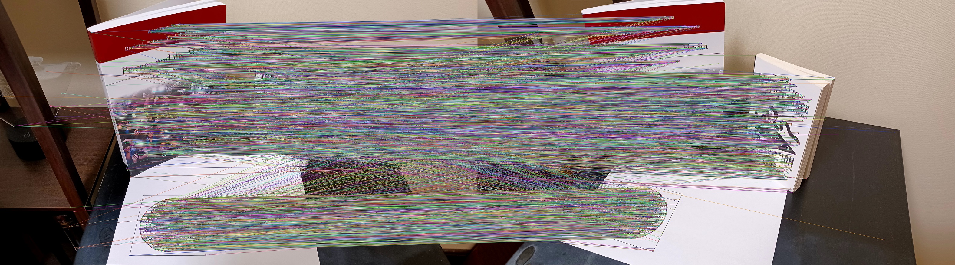
Likewise, the translation vector can either be the third column of the U matrix returned from SVD of the Essential matrix, or the negative of the third column. In order to determine the correct configuration of the rotation matrix and translation vector we simply test the possible configurations of rotation matrices and translation vectors and select the combination that produces the point in front of both camera positions using point triangulation. Once the relative rotation matrix and translation vector are recovered, they can be used in the following step to recover the depths of the keypoints in the first image. Epipolar constraints are applied the same way as previously described in this section to filter out bad matches between image pairs. The two images below show an example of epipolar constraints filtering out keypoint matches that did not satisfy the constraint.
Once the matches between two images have been filtered, we can begin to recover the depths of the keypoints from the perspective of the first image in each pair. We know from the previous sections that the relative rotation and translation parameters between the to image pairs can be used to describe a point from the first image on the second image. This relation can then be decomposed into vectors in camera space with scalar depth values represented by lambda. This expression can be written as follows:


Where lambda prime refers the depth of the second image’s point (p’) and lambda refers to the depth of the first image’s point (p). Gamma in this case should be 1 which is a property we will use to normalize the depth values we compute using SVD. We can further rearrange the terms in the expression to take the form of a minimization problem with which we can apply SVD. Thus, the expression can be written in matrix vector form to solve for the depth values of the point associated with the first image by taking the cross product of p’ on both sides of the equation. This will give us the following matrix vector relationship.

Given n matched features between the two images, we construct the matrix in the relationship Ax=0 where A holds the terms of our linear expressions and x is the list of unknown depths and gamma as the last term, which will be used as a normalization term after SVD. The matrix A is constructed as follows:

We then perform singular value decomposition on the matrix A to solve the minimization problem.

We use the last row of the Vt matrix, which consists of the orthonormal eigenvectors of the product between the transpose of the A matrix and A. The reason we use the last row is because it contains the solution which solves the minimization problem since the eigenvalue associated with the last row of Vt is the one closest to 0. The length of this solution vector is n+1, the last term being gamma so to compute the depths we divide all values in the vector by the last term in the vector, which now produces a gamma of 1.
The depth values computed in the previous section correspond with the matched features used in the diagonal of the A matrix. The depth values are multiplied accordingly with the normalized feature coordinates (in camera coordinate space) to recover the depths for each feature in image 1.

Where x is the homogenous, normalized coordinate of the feature in image 1 (in camera coordinates) and lambda n is the previously computed depth that corresponds with feature n from image 1. This produces the 3D coordinate point X for feature n. These depths are stored as 3D numpy arrays which are processed into a 3D point cloud.
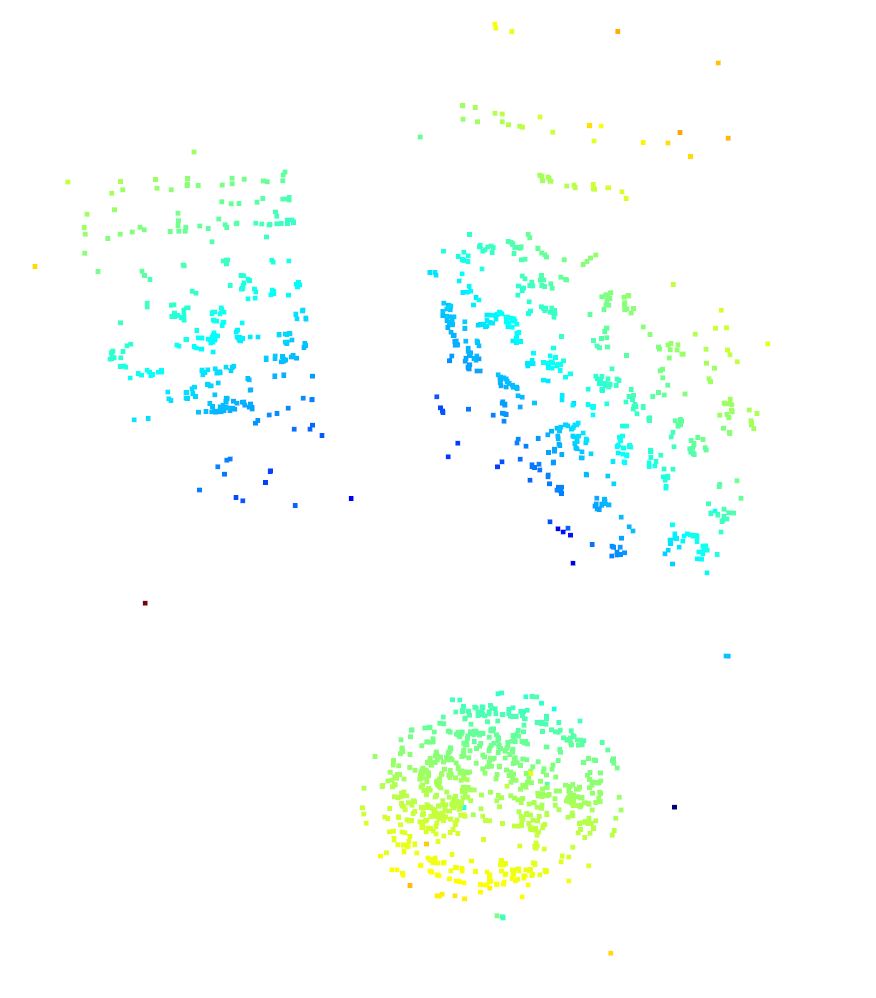
To generate the 3D point cloud, I use the open3d package in python and create a new PointCloud geometry object. I set the points parameter for the newly created PointCloud object to the list of 3D points computed in the previous section. Open3d then computes and displays the point cloud given those 3D coordinates, the results of which are viewable below.
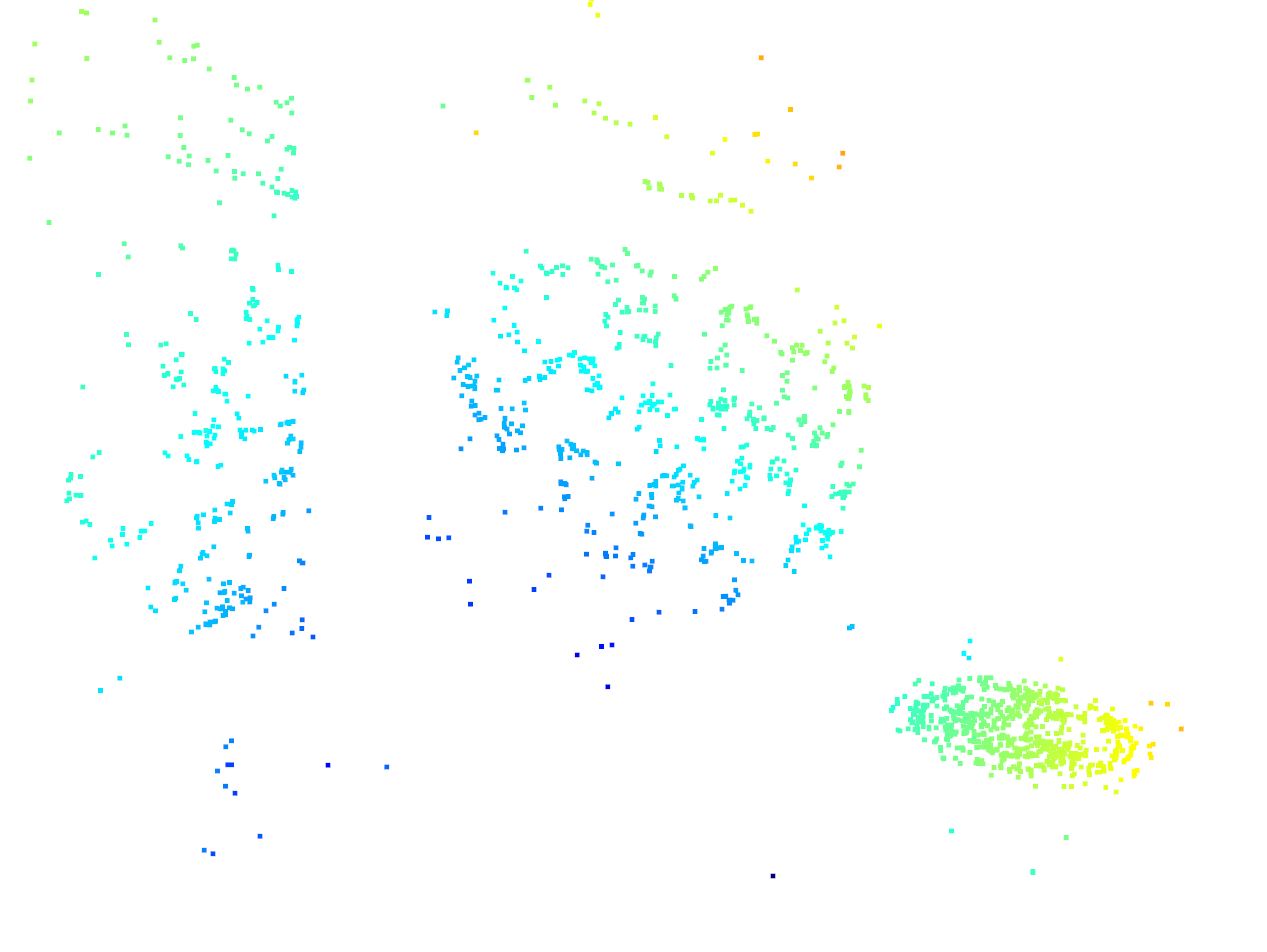
You can play the video below to get a better visualization of the 3D point cloud being explored.
This project consisted of an implementation for recovering 3D structures from 2D images taken on a smartphone. A key component of the process was calibrating the camera to acquire the new intrinsics matrix and undistort the images taken on the phone camera. Afterwards, two approaches were discussed with respect to recovering the relative rotation and translation transformations between image pairs. The first was to recover the homography of a known texture in the scene to acquire the world coordinate position of the camera with which the relative rotation matrix and transformation vector for each image pair could be computed. The alternative method was to use the 8-point algorithm to approximate the Fundamental matrix using SVD with which the Essential matrix could be recovered and decomposed to get the relative rotation and translation matrix for each image pair. These relative transformations are key to constructing the matrix used to recover depths from the first image in each pair. Once these depths are recovered using SVD, they scale the camera-space coordinates for each feature in the first image in an image pair and are then passed in as a numpy array to open3d where they are visualized as a 3D point cloud. By completing this project, I gained a much better understanding of epipolar geometry and an intuition of how 3D structures are recovered from 2D images taken from different centers of projection.