Erich Liang
Bells and Whistles Implemented:
- Part 2.2: Colored hybrid images
- Part 2.4: Colored multiresolution blending
|
|
|
|
|
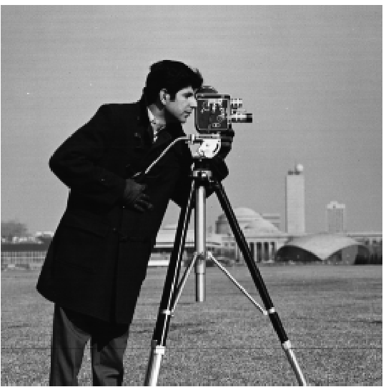
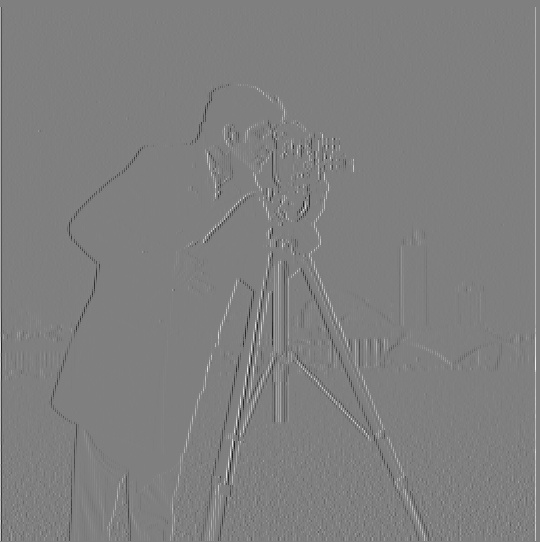
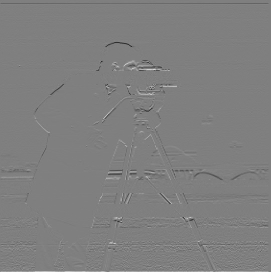
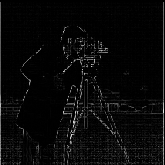
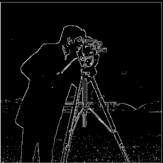
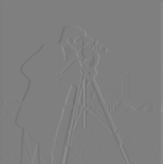
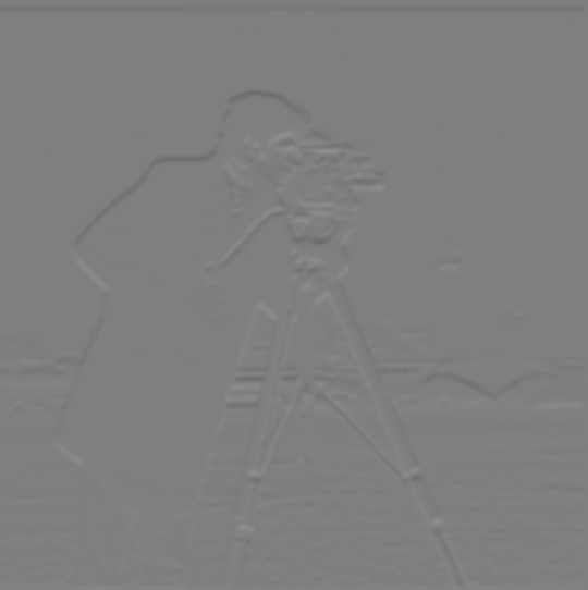
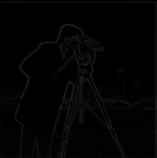
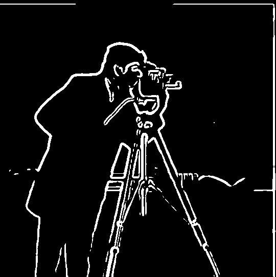
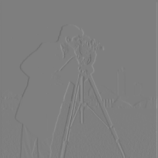
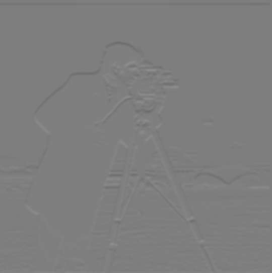
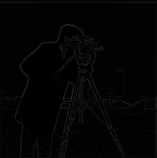
| Original Image | Partial Derivative in X | Partial Derivative in Y | Gradient Magnitude Image | Edge Image (threshold 0.1875) |
First, I computed the partial derivative of the image with respect to x and y directions; this was done by changing the scale of the original image's pixels to range from 0 to 1, and then applying convolution with the finite difference filters. Then, for each pixel, I took the square root of the sum of the pixel's partial derivative in X squared and the pixel's partial derivative in Y squared. I then scaled the resulting values back to range from 0 to 255, resulting in the gradient magnitude image.
 |
 |
 |
 |
 |
| Blurred Image | Partial Derivative in X | Partial Derivative in Y | Gradient Magnitude Image | Edge Image (threshold 0.06) |
By blurring the image first, we reduce the noise present before performing computing partial derivatives and the gradient magnitude image. As a result, the gradient magnitude image has much less noise compared to before, which allows for a much lower threshold to be used to form the edge image, as well as a much sharper and less noisy edge image. However, the edges detected are thicker compared to the edges detected without the blurring.
Instead of first blurring the original image and then applying the finite difference operators to it, we can instead directly use the convolution between the original image and derivative of Gaussian filters.
 |
 |
| DoG_x | DoG_y |
|
 |
 |
 |
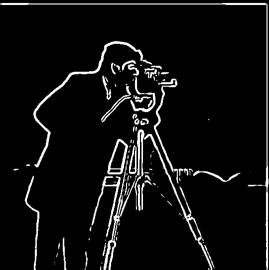 |
| Original Image | Partial Derivative in X (via DoG_x) | Partial Derivative in Y (via DoG_y) | Gradient Magnitude Image (via DoG) | Edge Image (threshold 0.06) (via DoG) |
As we can see, this results in basically the same edge detection. There are some slight differences, but this can be attributed to the fact that we are taking an approximation of the true derivative by using finite differences.
| Original Image | Sharpened Image |
 |
 |
 |
 |
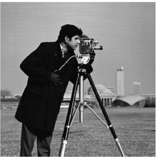
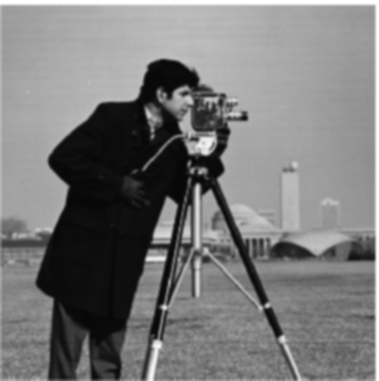
To evaluate the process, here is the original cameraman image, blurred, and re-sharpened version.
| Original Image | Blurred Image | Sharpened Image |
 |
 |
 |
In the process of taking the cameraman image, blurring it, and resharpening it, the blurred image is visibly blurrier compared to the two other images. The sharpened image has similarly well-defined edges compared to the original, but it is not an exact copy of the original image either. Specifically, there seems to be more noise overall in the sharpened image, and edges seem to have slightly higher contrast than before (some black edges seem to "glow white" around them).
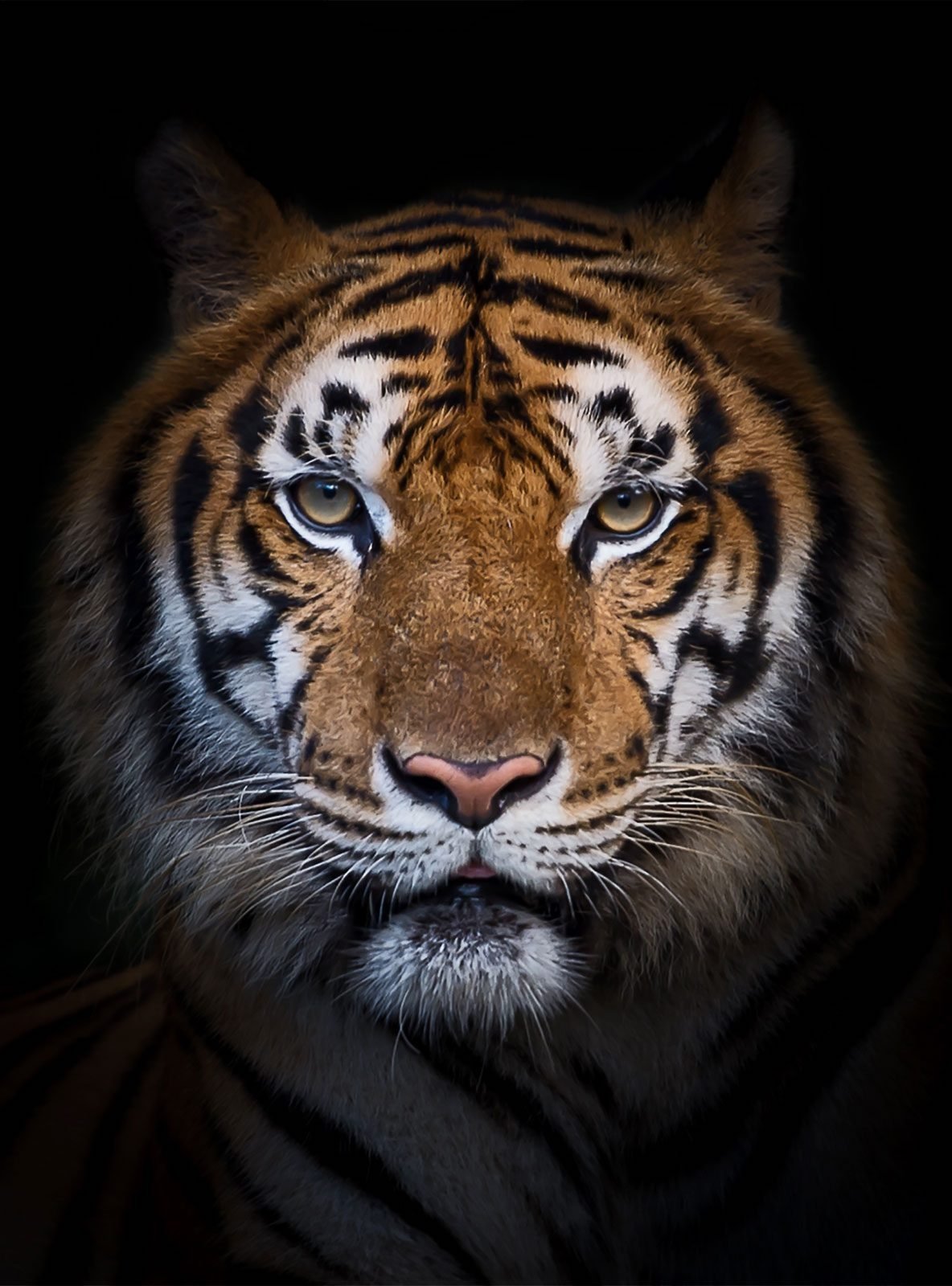
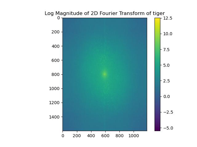
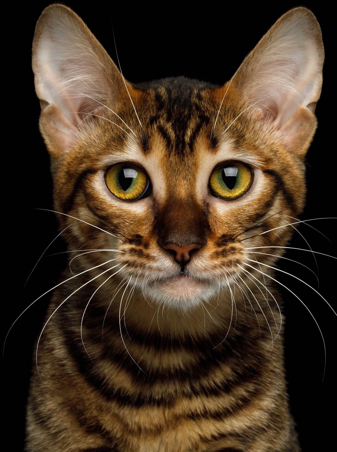
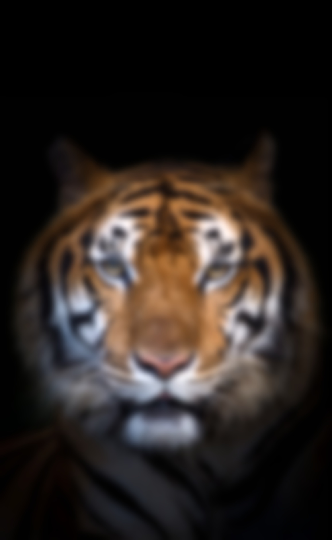
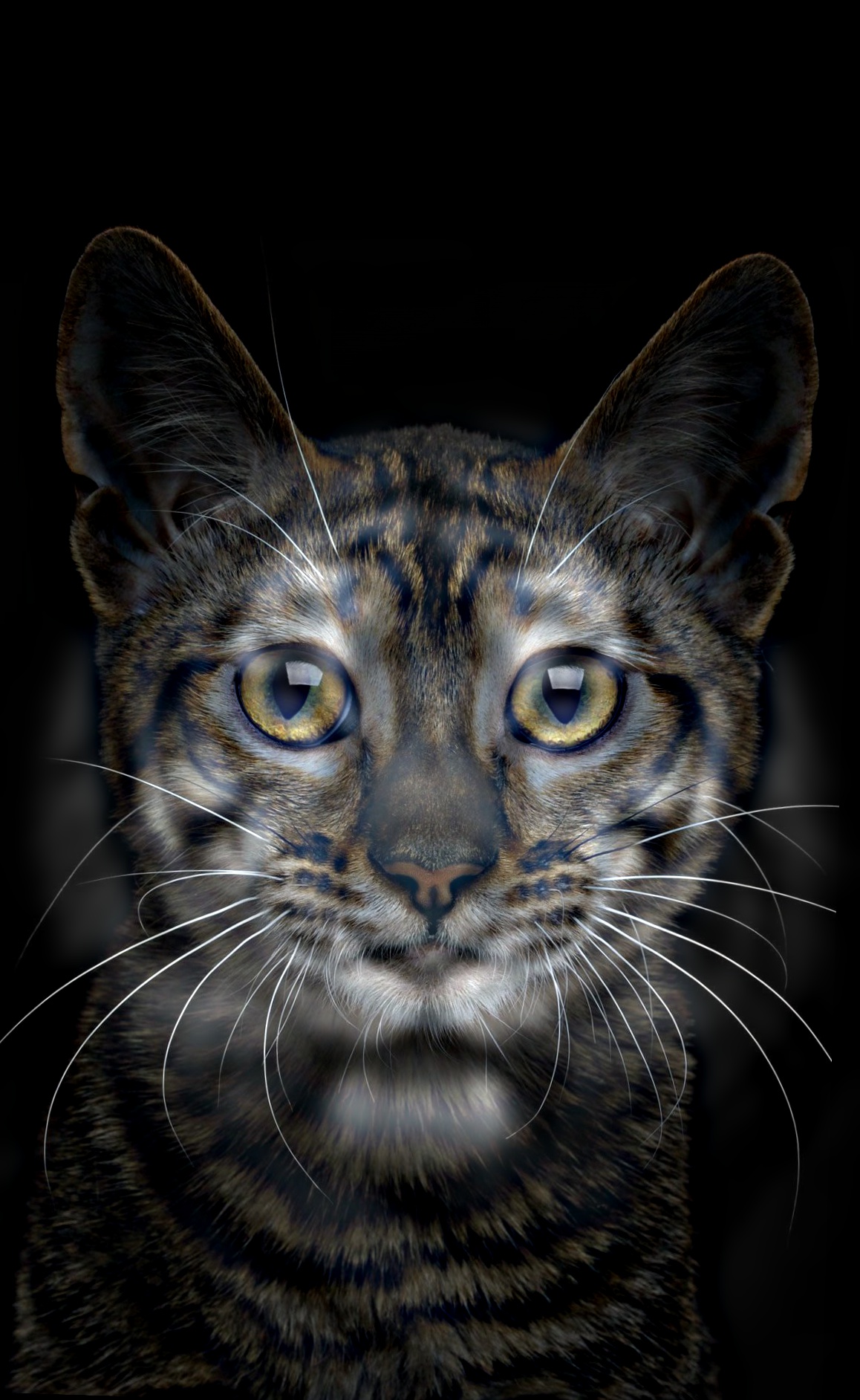
Here is a walkthrough of an example hybrid image, along with log magnitude of Fourier transform plots. Note that most of these images dynamically change size acording to window size. As a result, changing the percentage zoom of the website might not work well for viewing hybrid images, but resizing the web browser window size might do the trick. Please download and view locally for best results.
 |
 |
 |
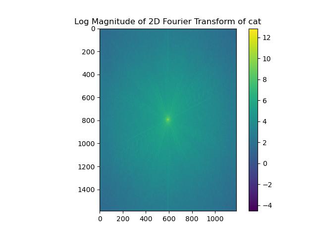 |
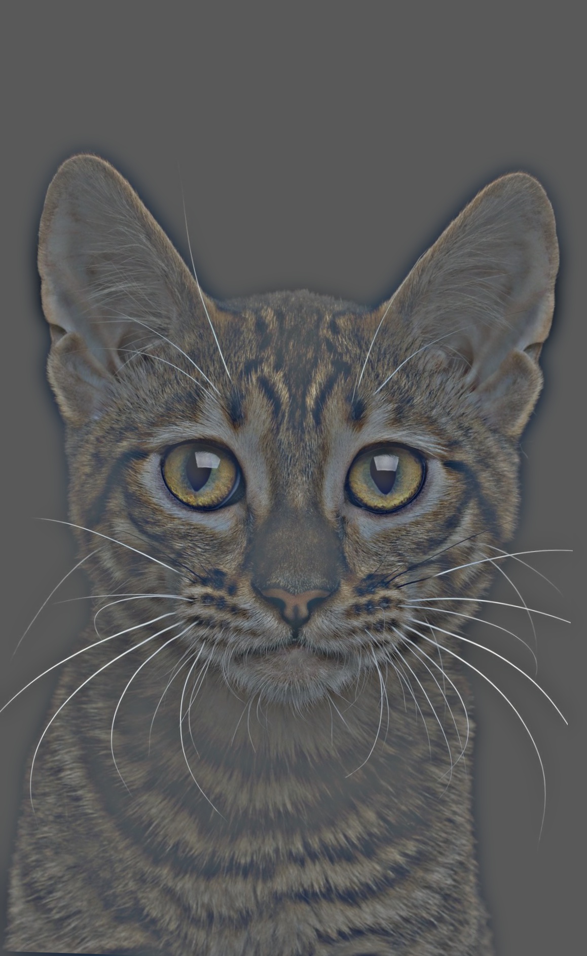
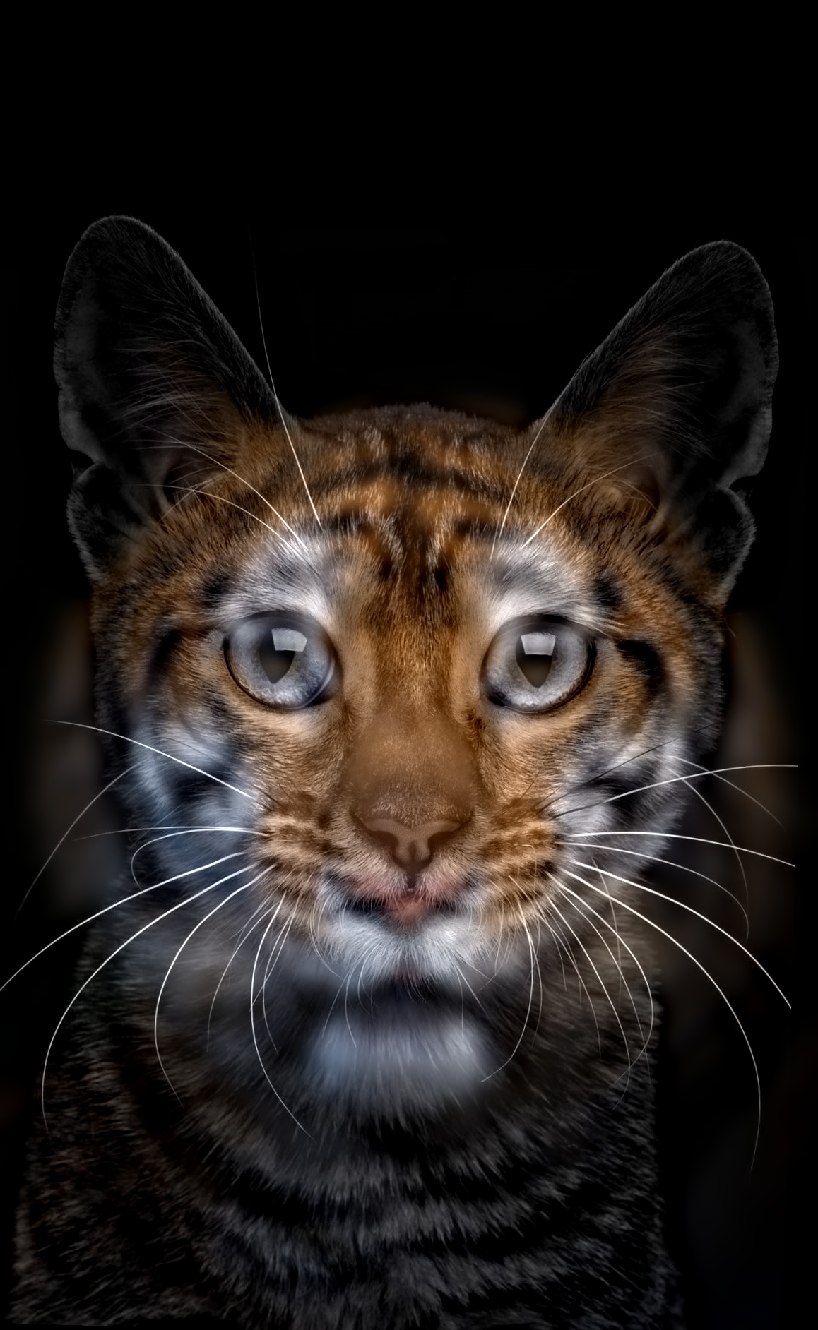
| Image 1: Tiger | Image 1 Log Magnitude FFT | Image 2: Cat | Image 2 Log Magnitude FFT |
 |
 |
 |
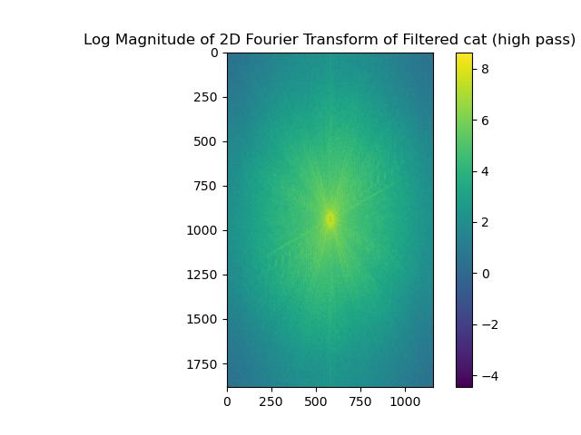 |
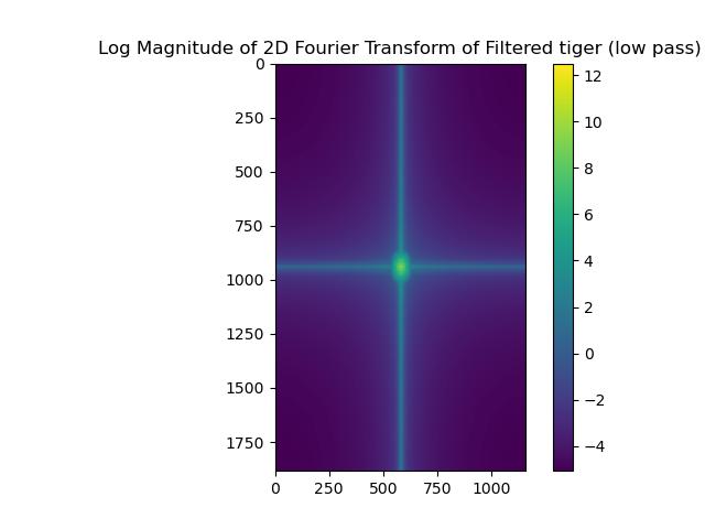
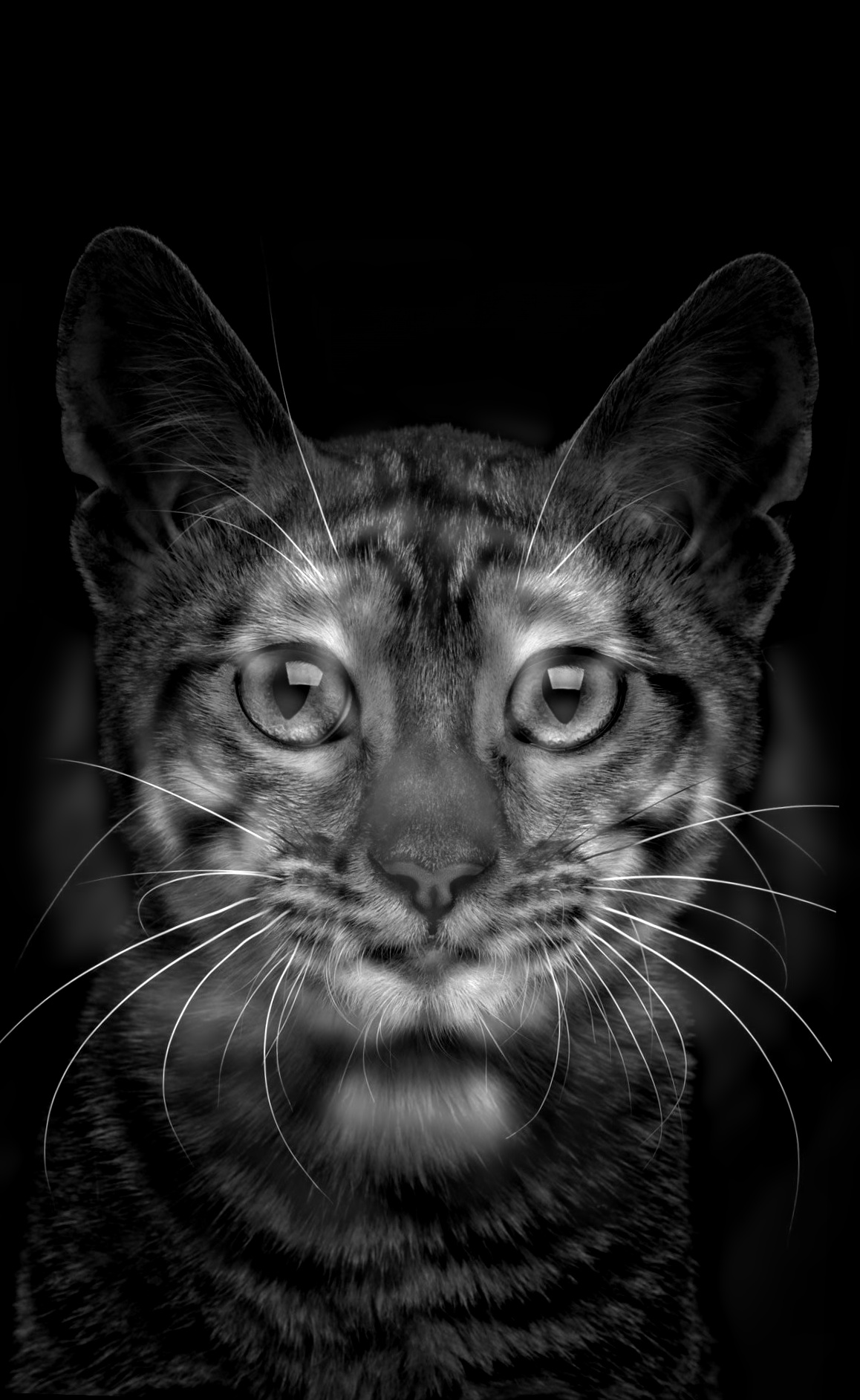
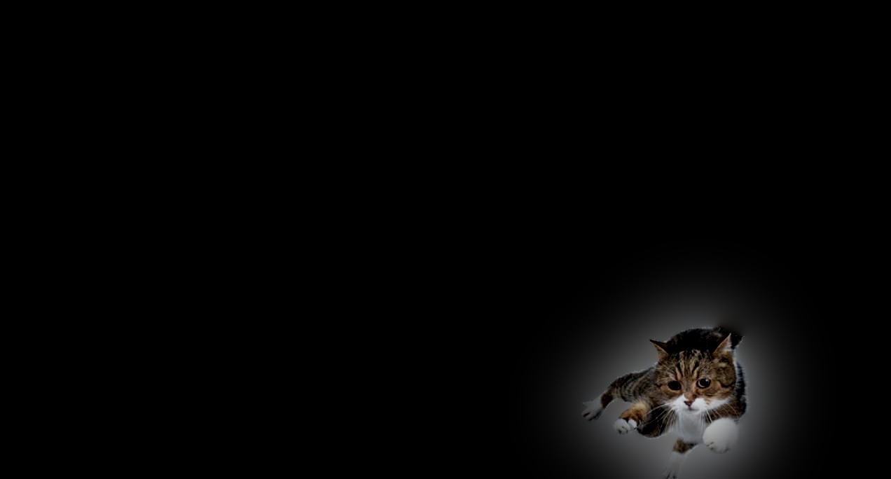
| Low Pass Filtered Image 1 | Low Pass Filtered Image 1 Log Magnitude FFT | High Pass Filtered Image 2 | High Pass Filtered Image 2 Log Magnitude FFT |
 |
 |
||
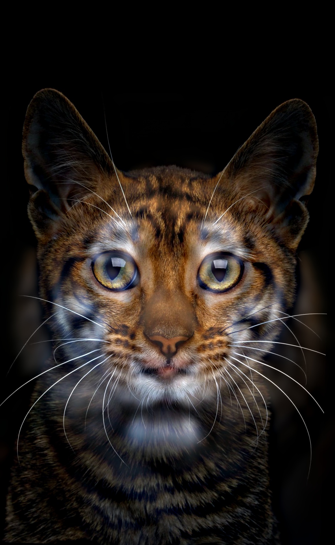
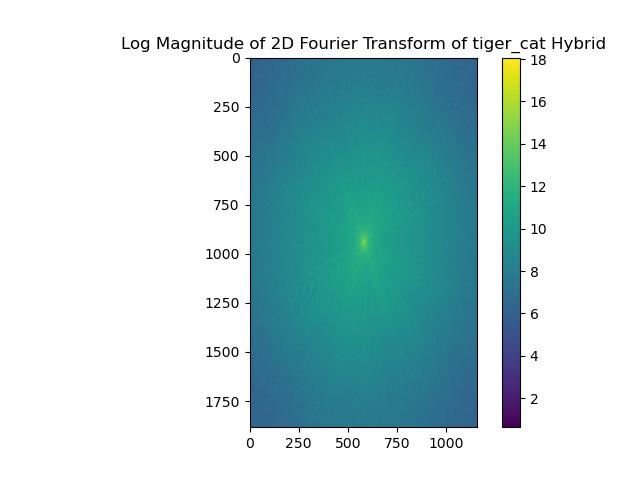
| Hybrid Image: Tiger/Cat | Hybrid Image Log Magnitude FFT |
Note that I have implemented color for the hybrid image formation. I also ran a few experiments about using color or grayscale images for the low-frequency component and high-frequency component. Below is an example of all 4 combinations. I personally found that using color for both low and high frequencies typically yielded the best-looking images, so for all the other examples I have, I used color for both low and high frequencies.
|
 |
 |
 |
| Colored Low Frequency, Colored High Frequency | Gray Low Frequency, Colored High Frequency | Colored Low Frequency, Gray High Frequency | Gray Low Frequency, Gray High Frequency |
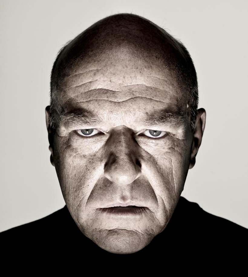
Here are a few more examples of hybrid images.
 |
 |
 |
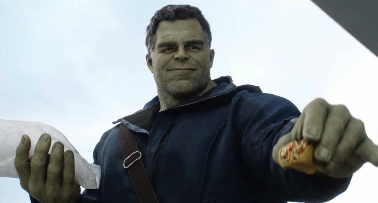
| Image 1: Happy, used as Low Frequency | Image 2: Angry, used as High Frequency | Hybrid Image: Happy/Angry |
 |
 |
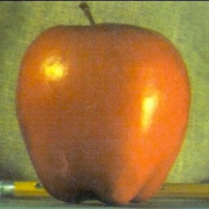
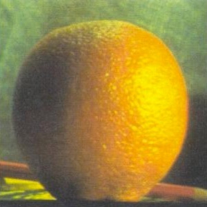
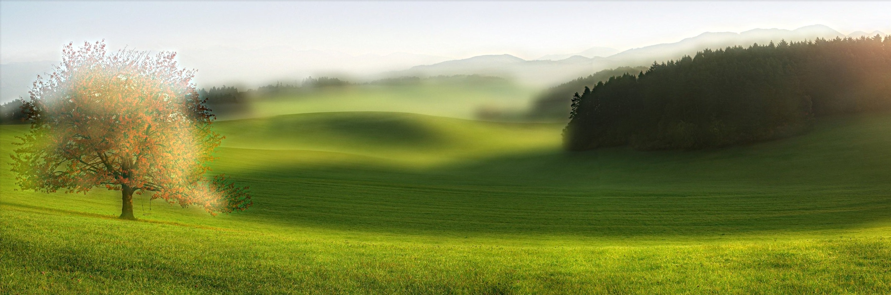 |
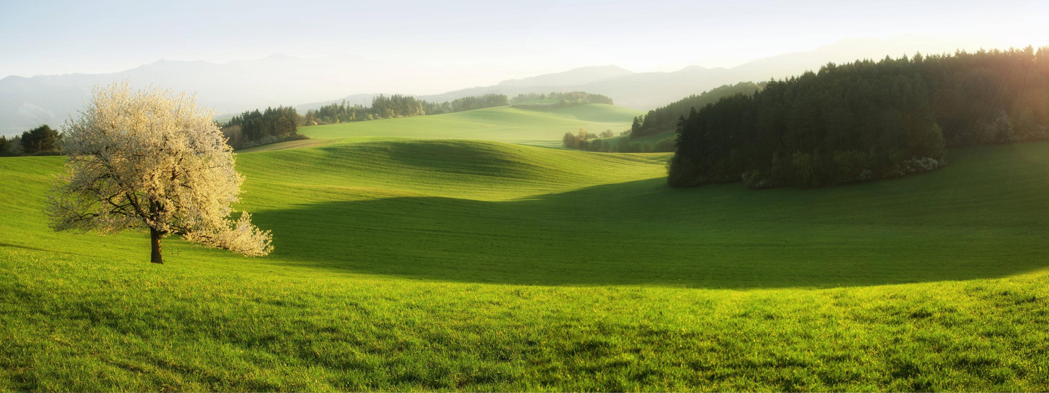
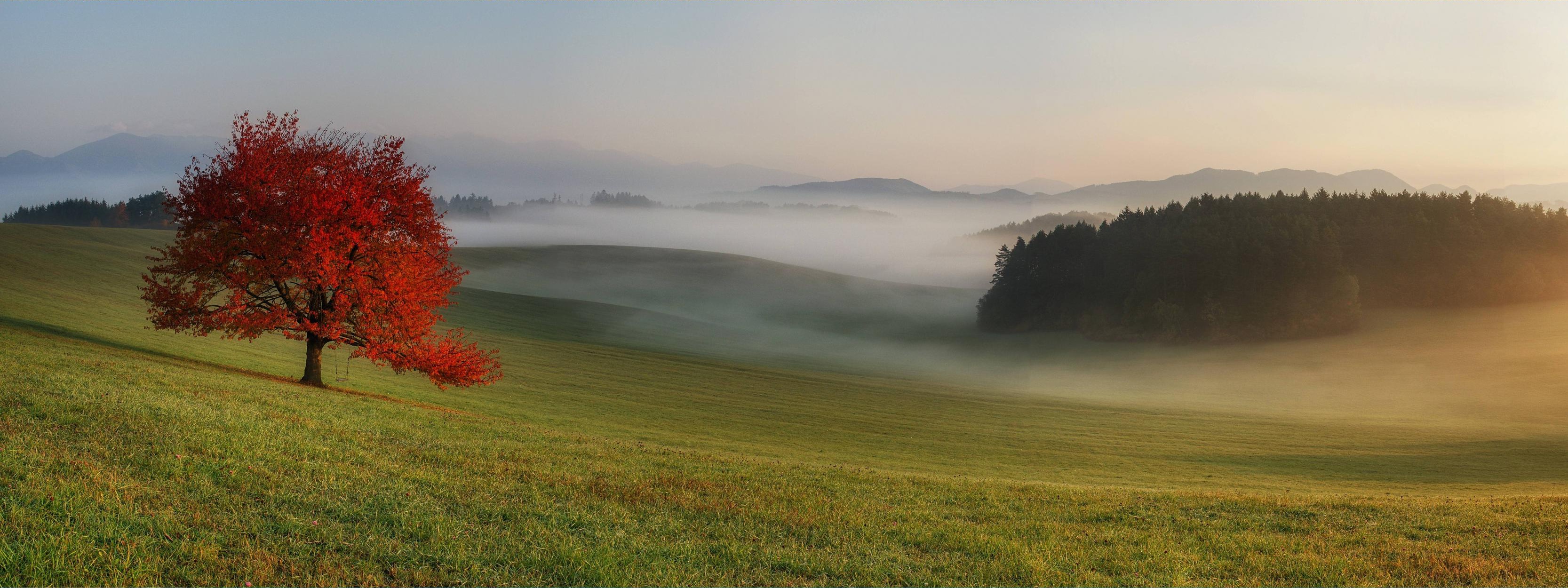
| Image 1: Spring, used as Low Frequency | Image 2: Fall, used as High Frequency | Hybrid Image: Spring/Fall (cropped) |
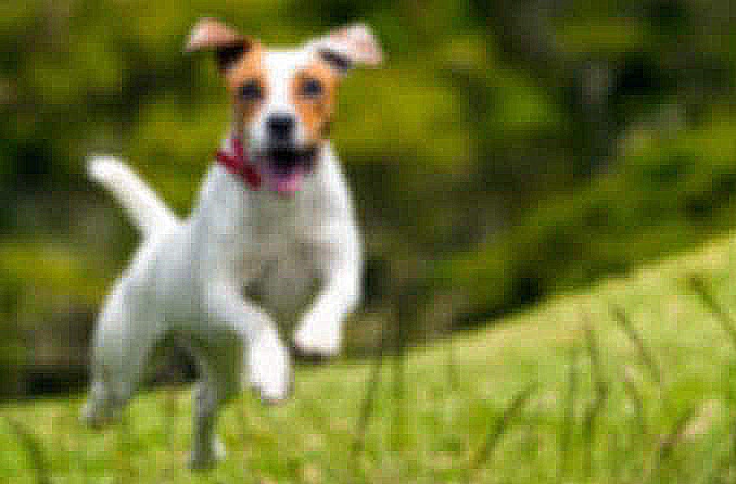
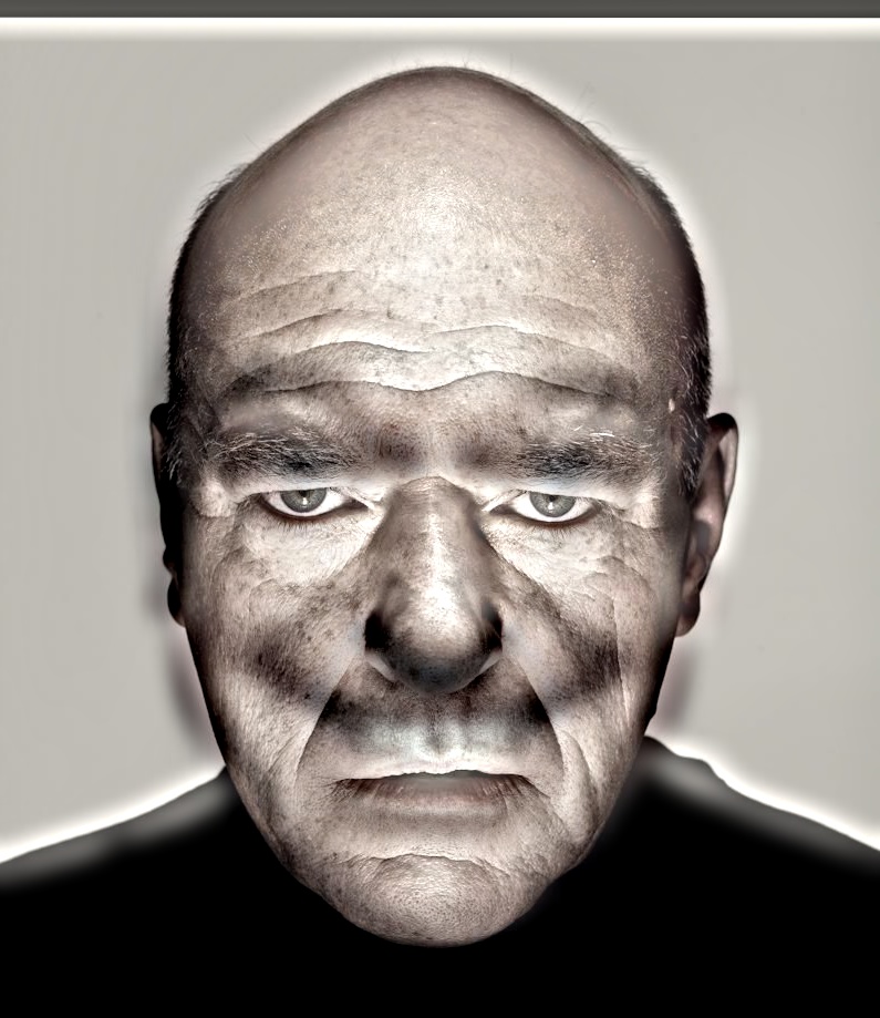
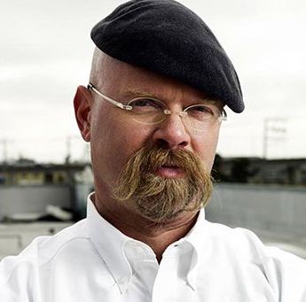
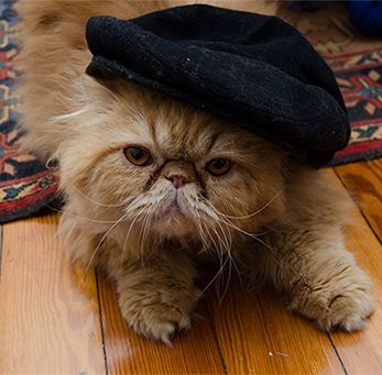
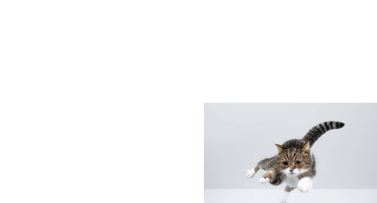
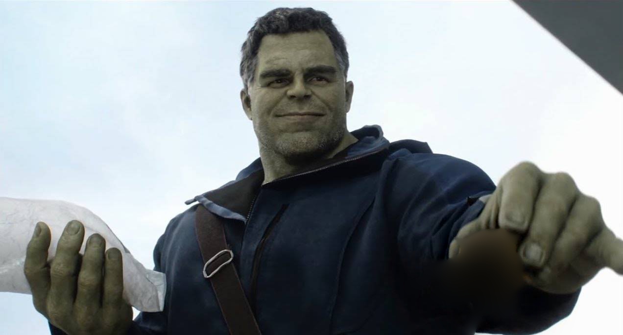
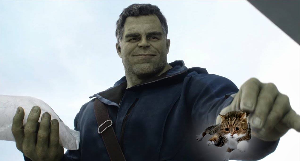
Finally, here is one more example of hybrid image that did not turn out as well as the rest. It still has the "hybrid" effect with the low and high frequencies, but the images were not aligned very well (aligning the hats results in the faces being misaligned, and vice-versa); hence, the final image doesn't look that coherent overall.
 |
 |
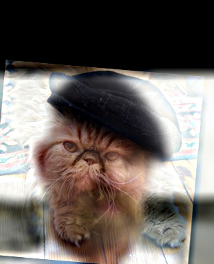 |
| Image 1: Jamie, used as Low Frequency | Image 2: Persian Cat, used as High Frequency | Hybrid Image: Jamie/Persian Cat |
Here is a replica of the Laplacian stack figure provided, but using my own implementation.
 |
 |
 |
 |
 |
 |
 |
 |
 |
 |
 |
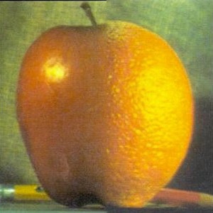 |
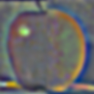
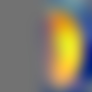
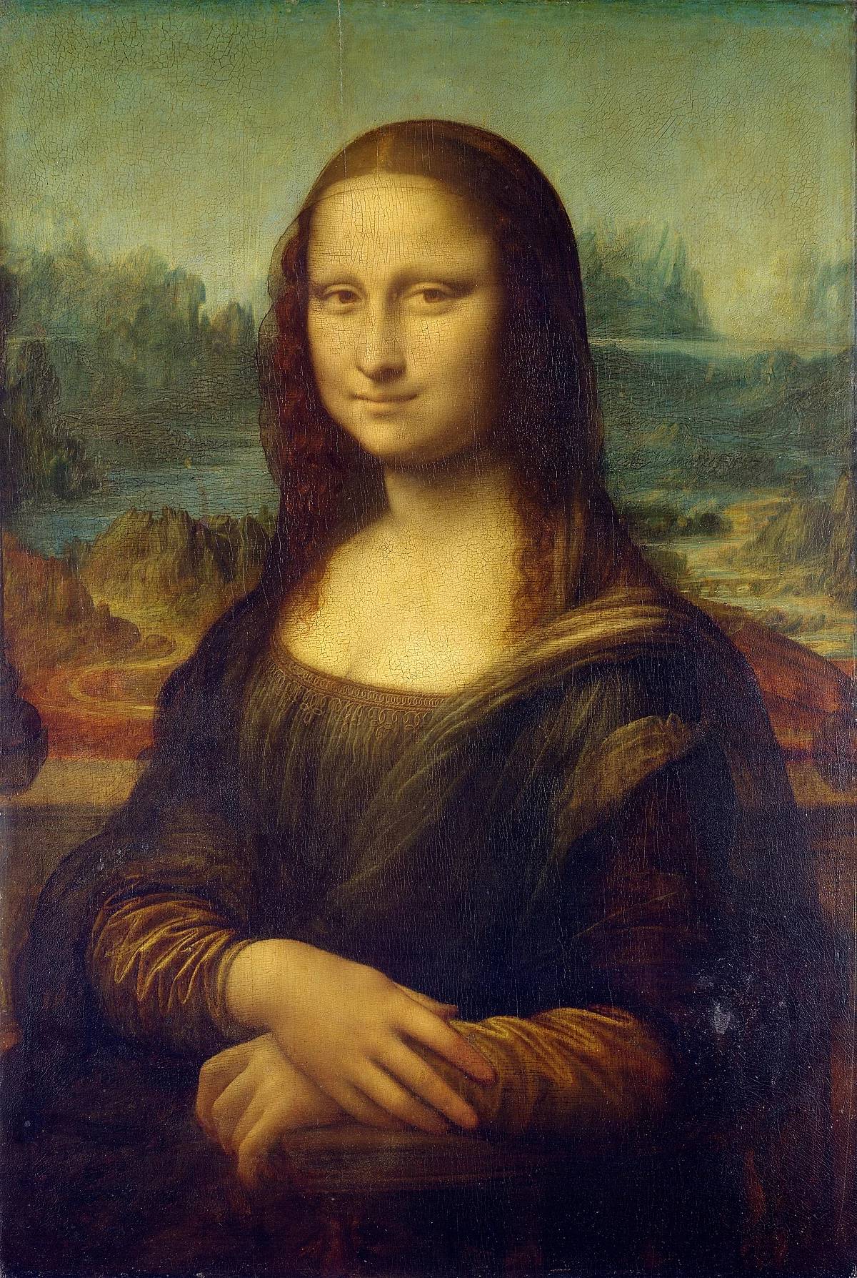
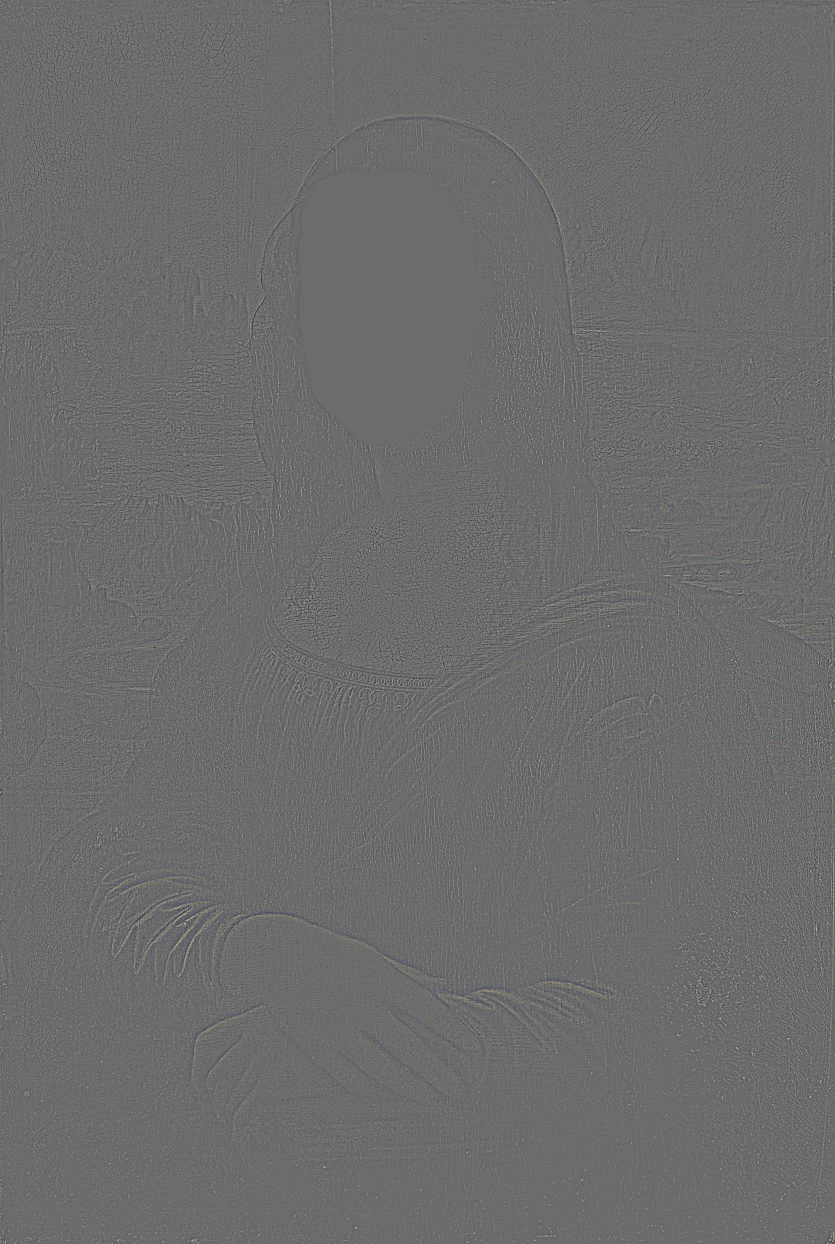
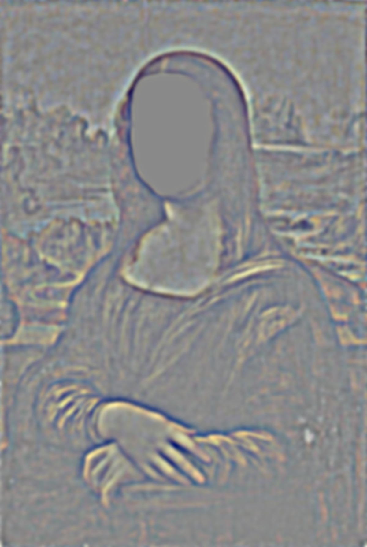
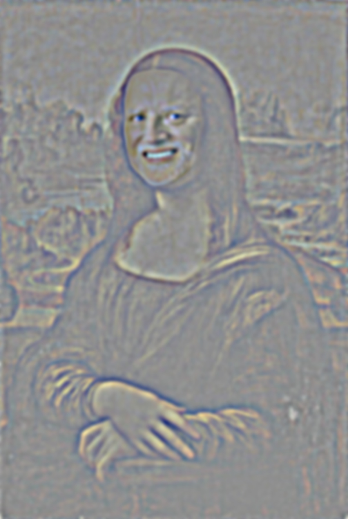
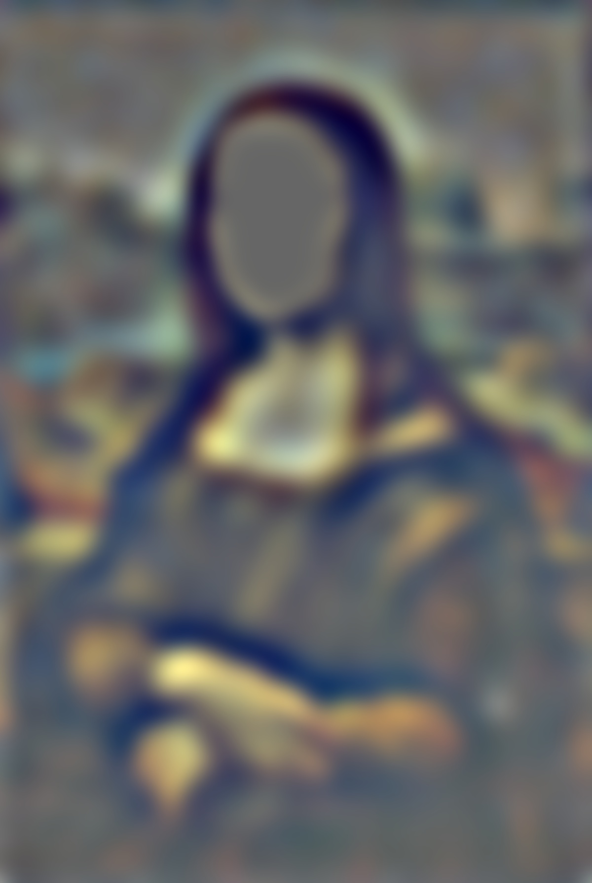
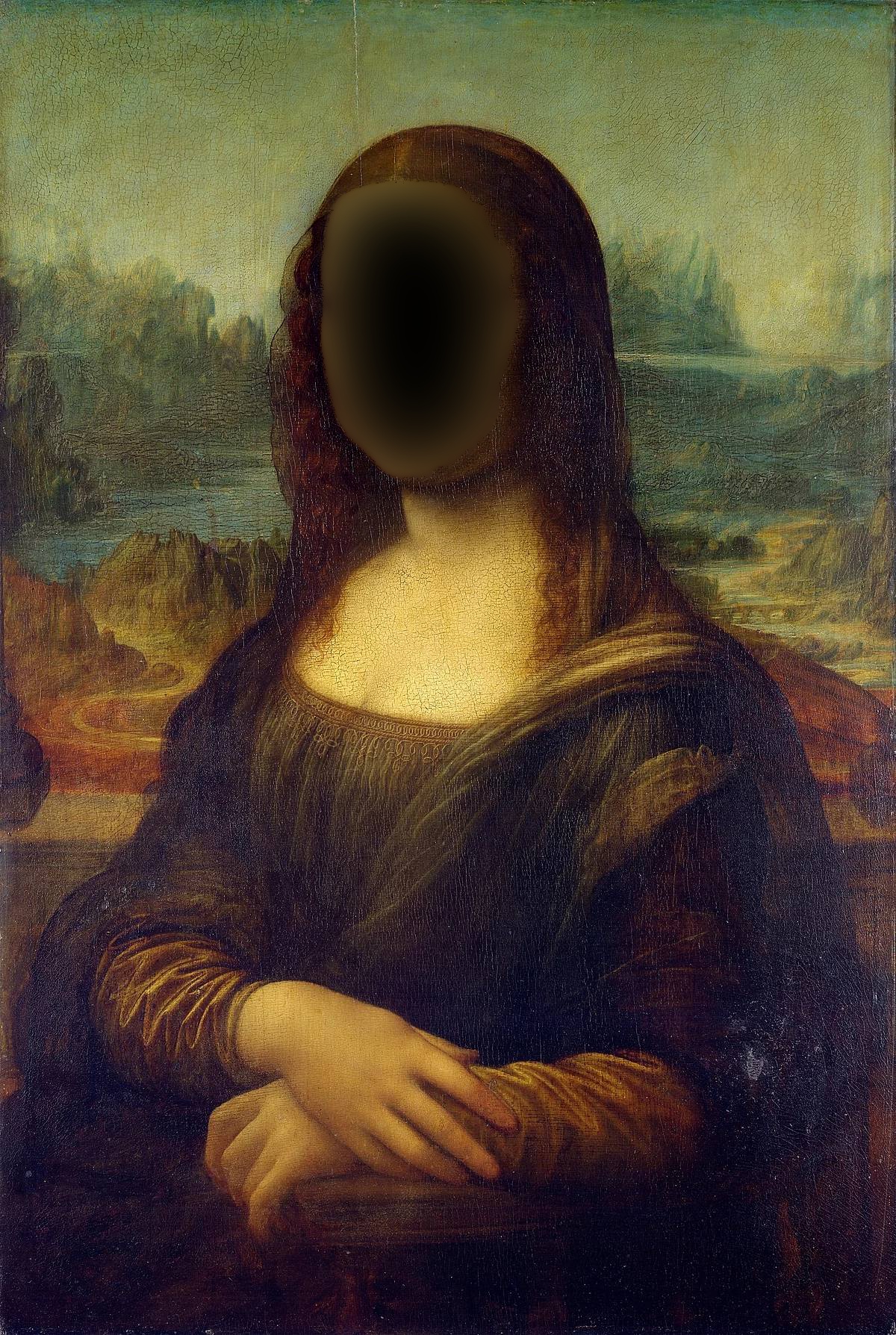
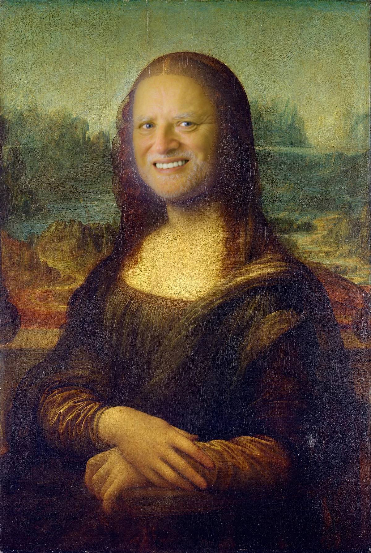
For one of my image blends, here is a showcase of original images, filters, and the laplacian reconstructions for the masked images and final blend image.
 |
 |
 |
| Image 1 | Image 2 | Binary Mask |
| Harold | Mona Lisa | Harold / Mona Lisa Blend | |
| Laplacian Stack Level 0 |  |
 |
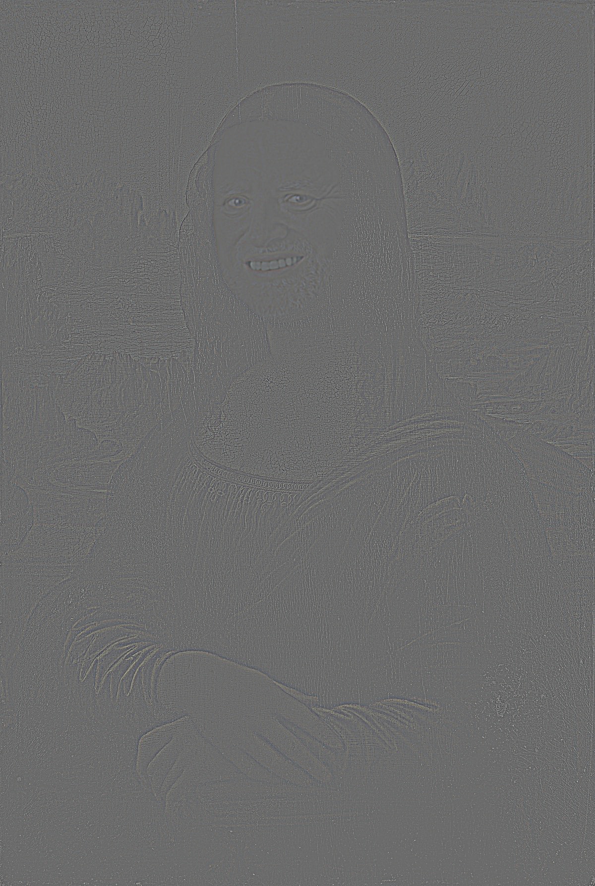 |
| Laplacian Stack Level 2 |  |
 |
 |
| Laplacian Stack Level 4 |  |
 |
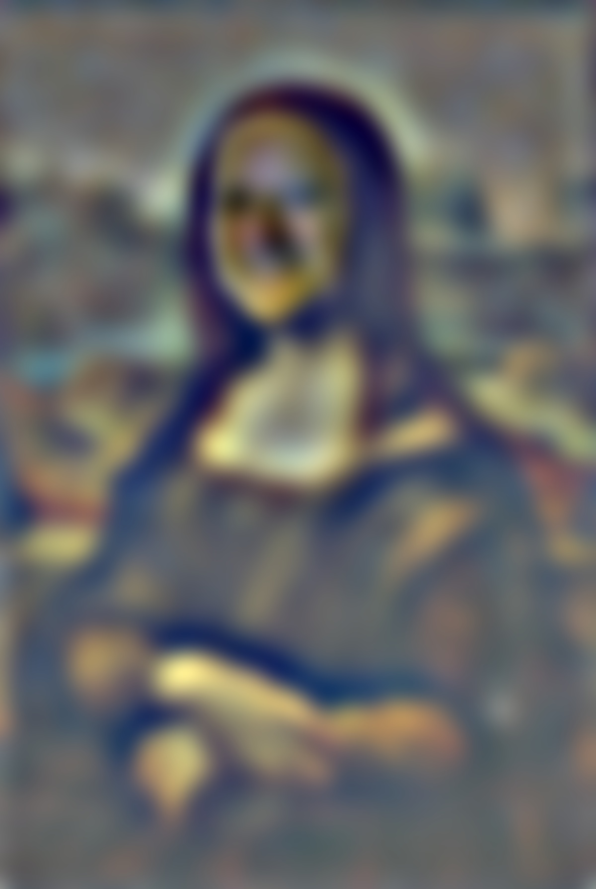 |
| Final Reconstruction | 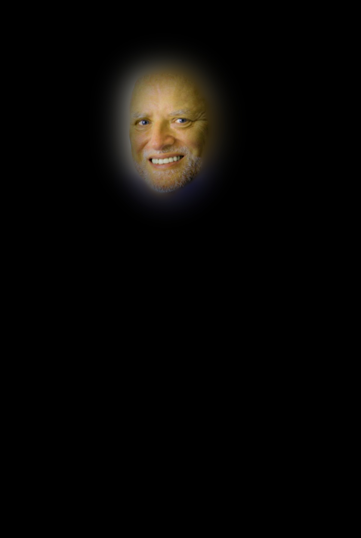 |
 |
 |
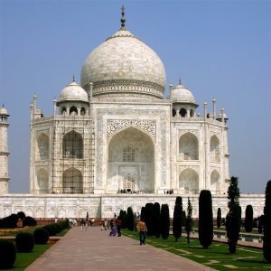
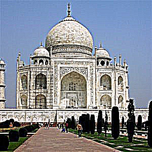
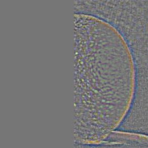
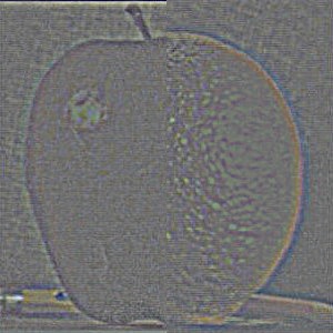
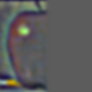
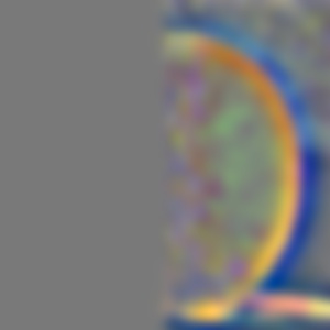
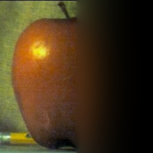
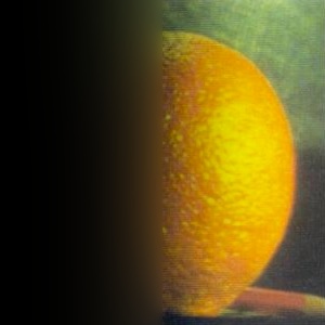
Here is a showcase of all the original images and final mutliresolution blend results I got.
|
|
|
| Image 1 | Image 2 | Binary Mask |
|
|
|
| Masked Image 1 Reconstruction | Masked Image 2 Reconstruction | Final Blend Reconstruction |
 |
 |
 |
| Image 1 | Image 2 | Binary Mask |
 |
 |
 |
| Masked Image 1 Reconstruction | Masked Image 2 Reconstruction | Final Blend Reconstruction |
 |
 |
 |
| Image 1 | Image 2 | Binary Mask |
 |
 |
 |
| Masked Image 1 Reconstruction | Masked Image 2 Reconstruction | Final Blend Reconstruction |
Overall, I had a lot of fun with this project! One of the important things I learned was that in order to get a good blending result (either through hybrid images or multiresolution blending), one really needs to get an aesthetically pleasing alignment of the two starting images.