Project 4 of UC Berkeley's CS194-26 course teaches us how to use neural networks to automatically detect facial keypoints using different neural network architectures. We first start by training a Convolutional Neural Network to detect the nose tip, gradually building up to identifying the full face via its keypoints.
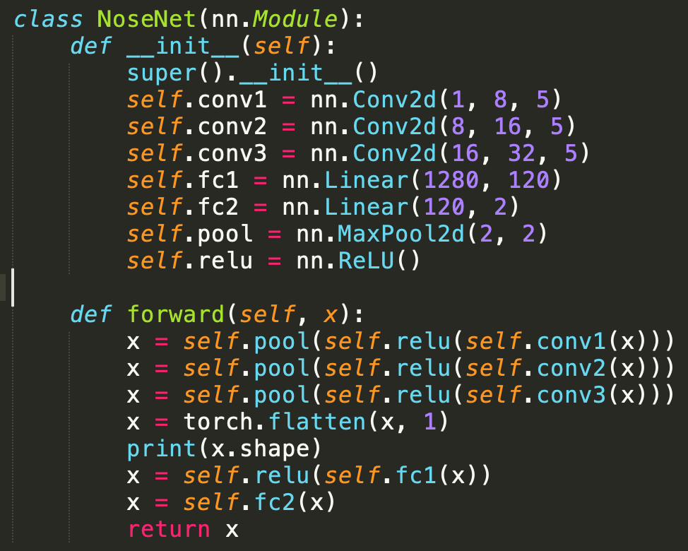
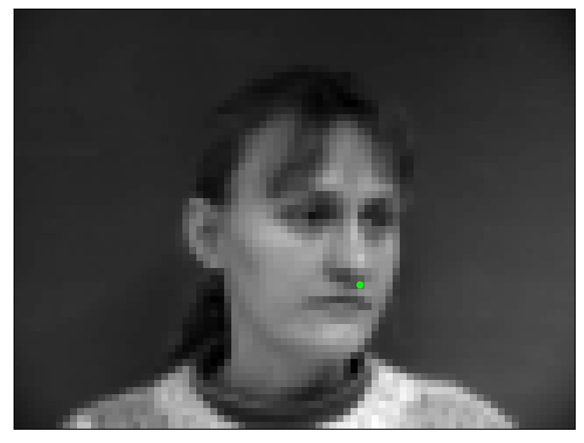
The first task is to identify the nose keypoint on an greyscale image. We cast the nose detection problem as a pixel coordinate regression problem, where the input is a single grayscale image, and the outputs are the nose tip positions (x, y). I used a CNN with the MSE loss function, a learning rate of 0.001, training for 25 epochs. The architecture is shown below
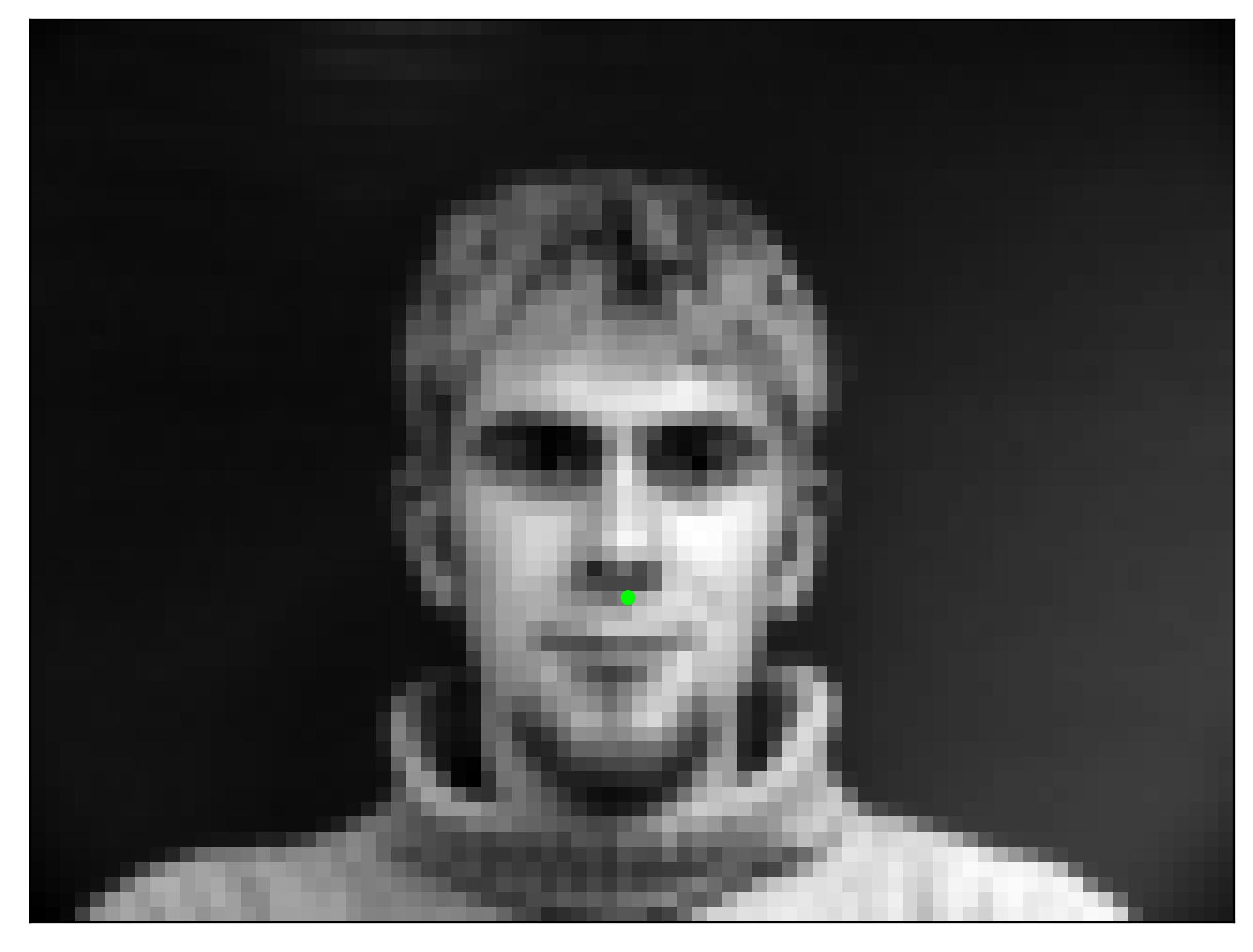
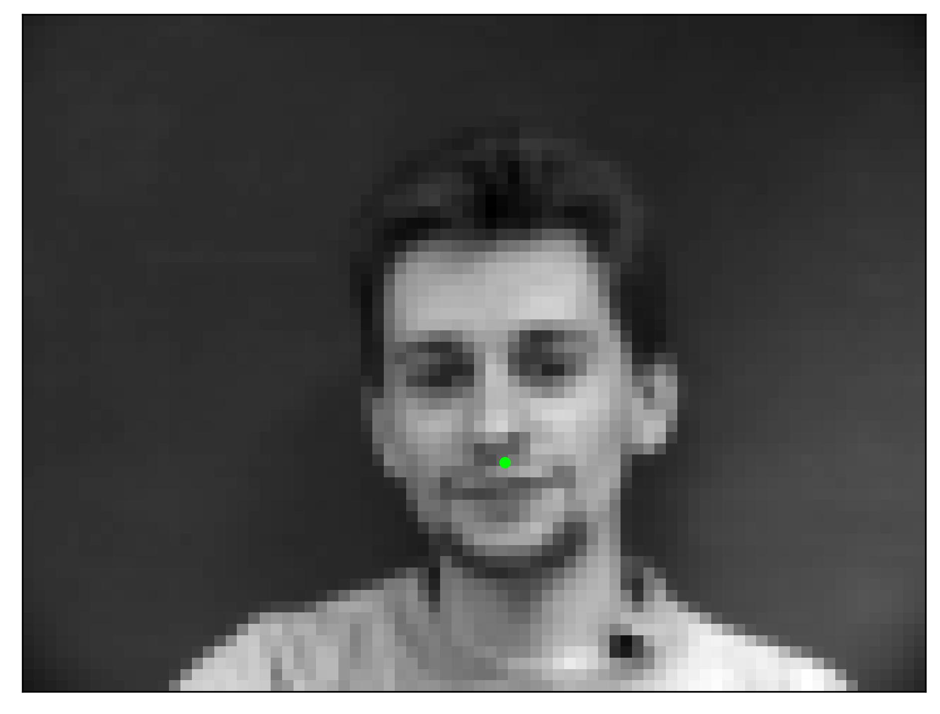
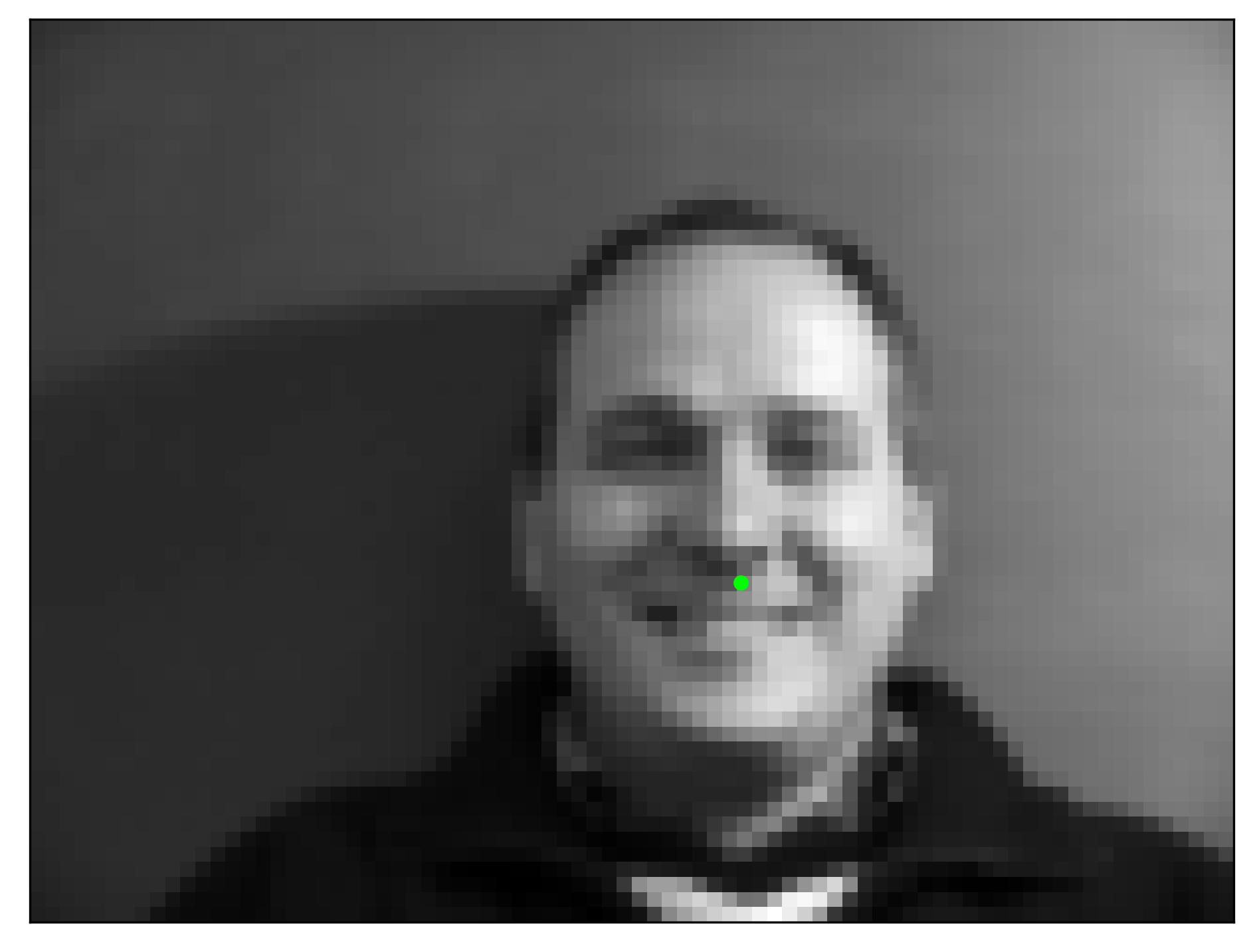
For all images in our data set, we convert each to grayscale and resize to (80, 60). Using the Pytorch DataLoader, a few sample images and their corresponding nose tips are shown below.
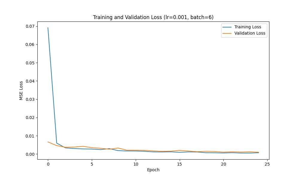
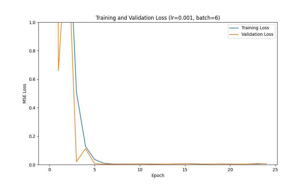
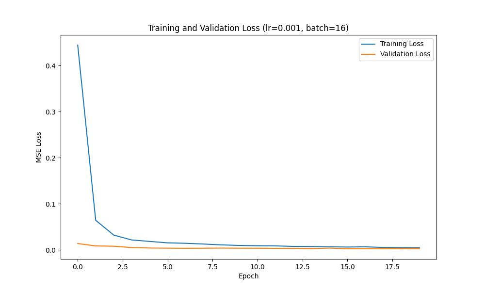
We can plot the training and validation loss curves across each epoch to show the training progress; such curves are shown below:
To show the effect that the hyperparameters (i.e. learning rate, batch size, kernel size) can have on the performance of the model, I tried several different learning rates and batch sizes. Overall, I found that a learning rate of 0.001 and a (5,5) kernel were the most effective.
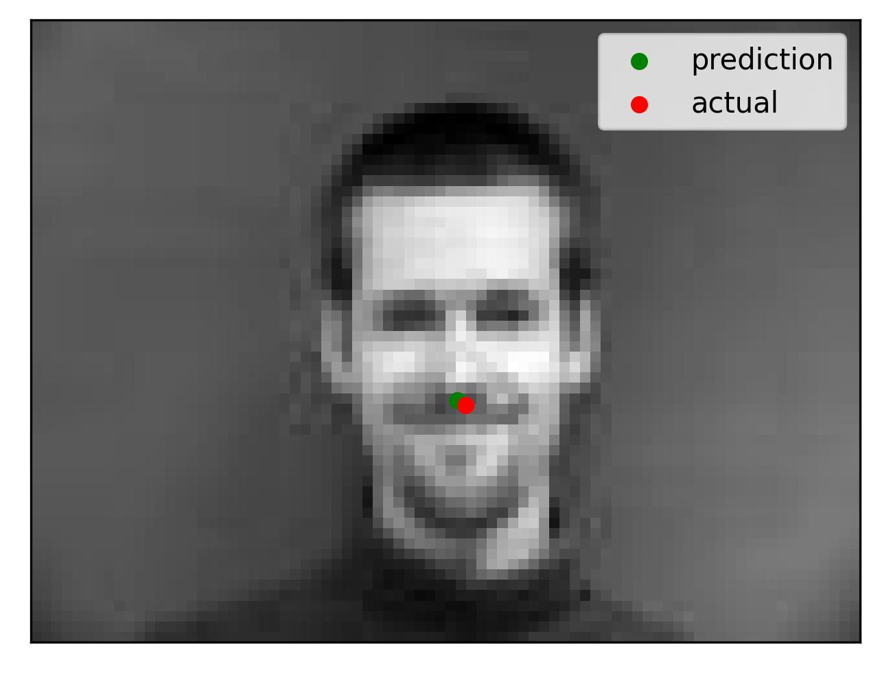
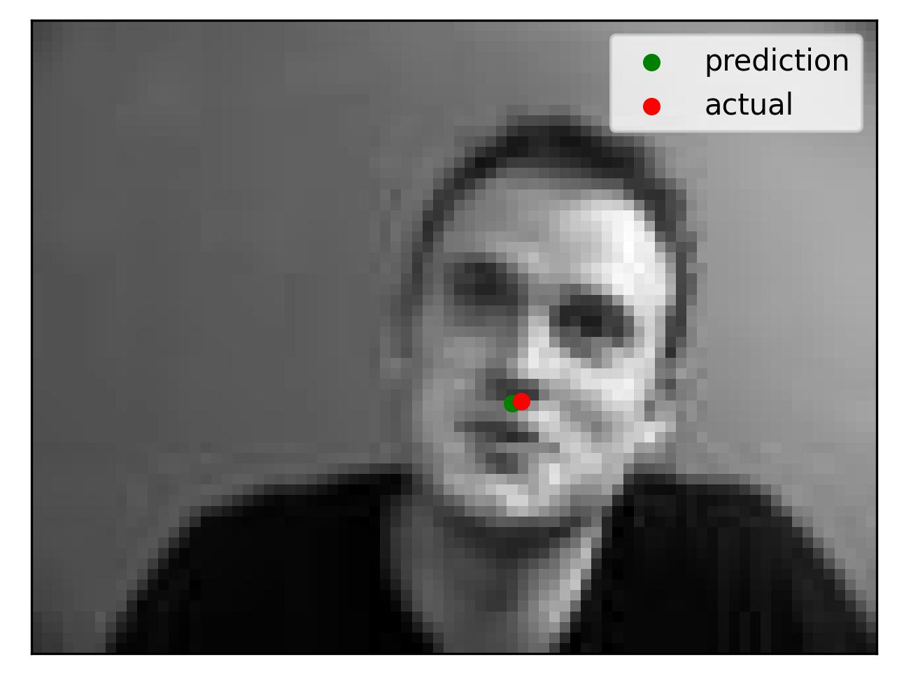
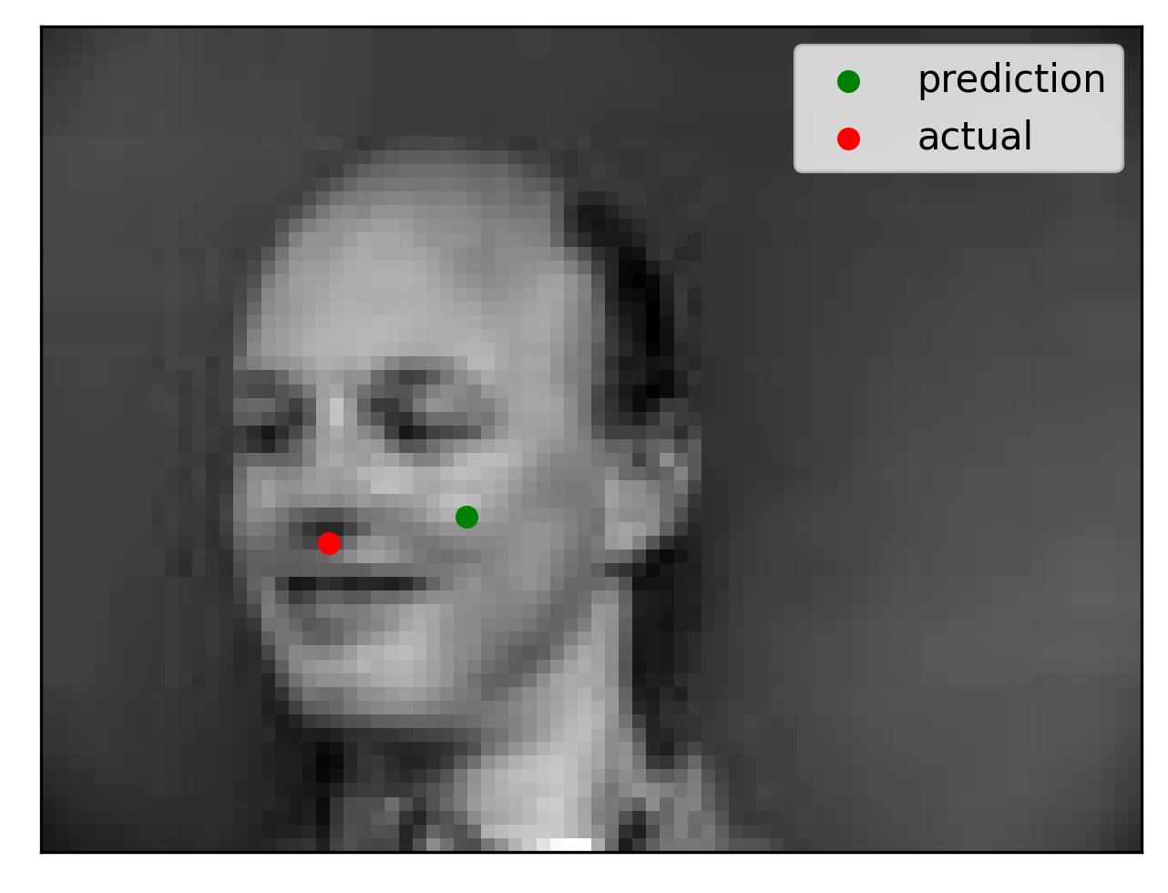
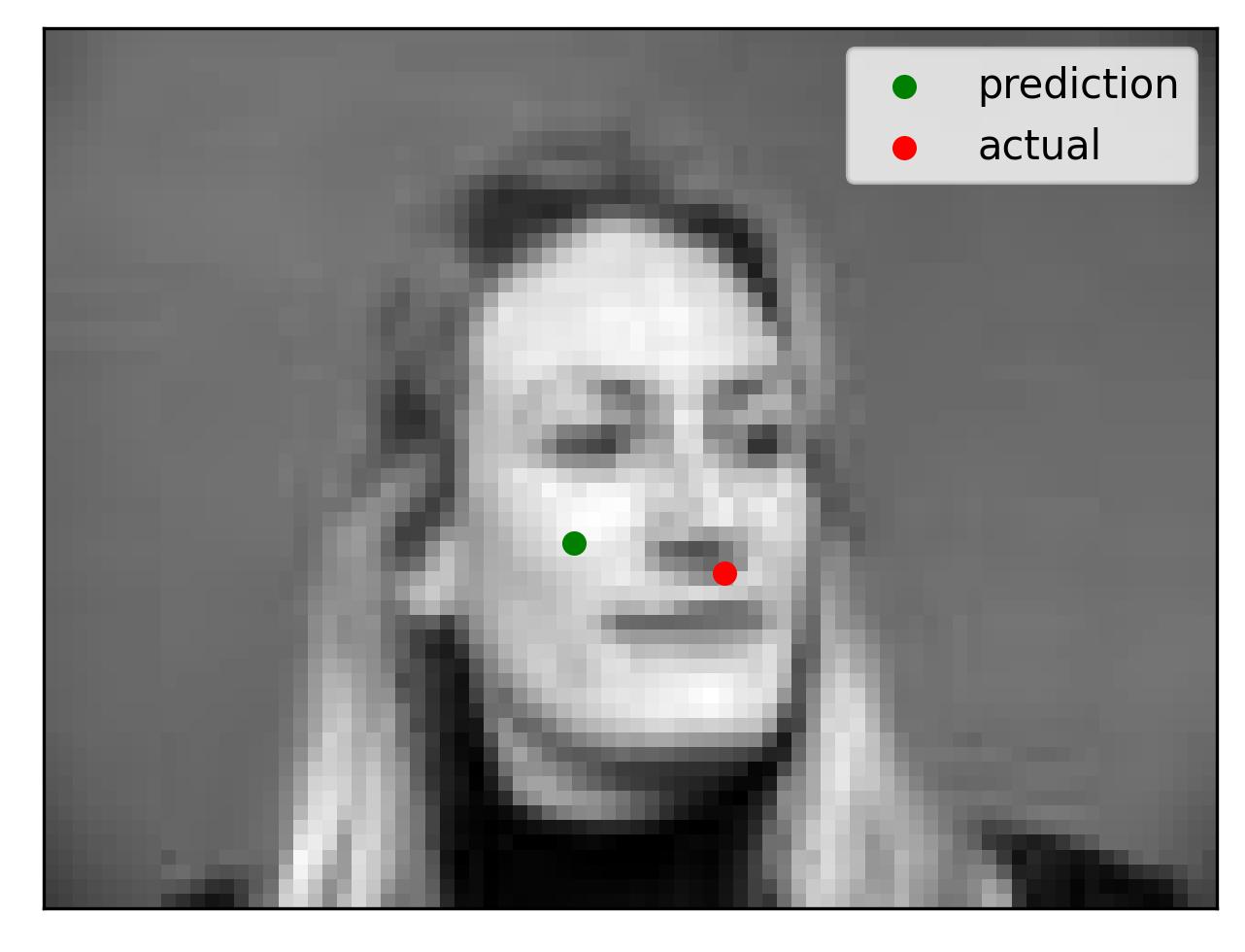
While my model performed well, there were examples in which it did not work well. Shown below are two failure cases and two successful cases.
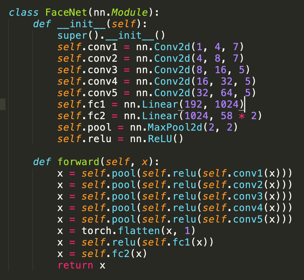
Building on the NoseNet, we extend our model to predict all the facial keypoints (not just the nose). The FaceNet consists of five convolutional layers followed by full connected layers. Each convolutional layer is followed by a ReLU and then a MaxPool with a size of (2,2) and a stride of 2. I used a learning rate of 0.001 and a batch size of 16, training for 25 epochs. I used MSELoss as the loss function and the Adam optimizer. The new architecture is described below:
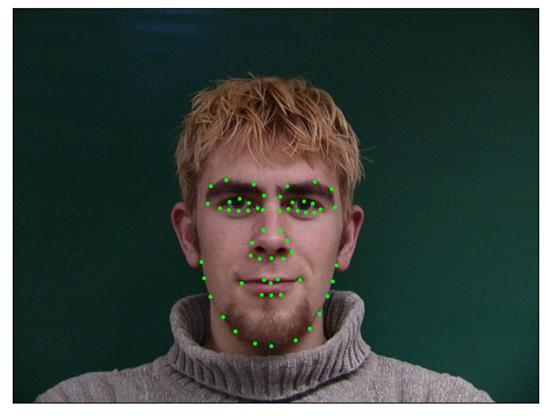
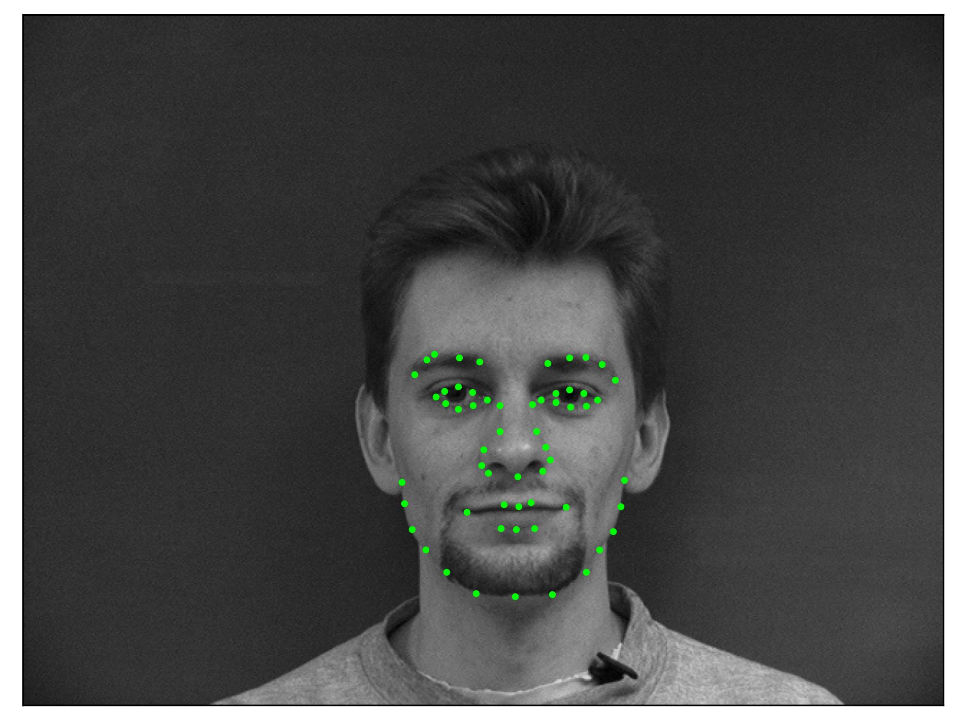
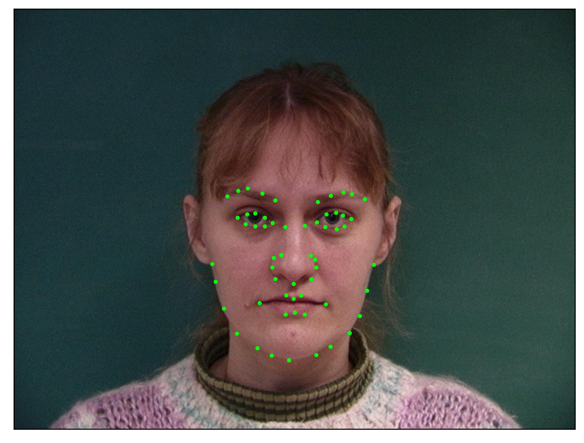
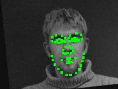
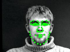
For all images in our data set, we convert each to grayscale and resize to (240, 180). Using the Pytorch DataLoader, a few sample images and their corresponding facial keypoints are shown below.
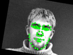
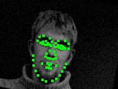
To avoid overfitting, I applied a series of data augmentations to the rescaled images. For each image, I rotated the image and keypoints a random angle between -15 and 15 degrees, horizontally flipped the image with a low probability, added some random Gaussian noise, and changed the brightness by some random amount. Some augmented images are shown below.
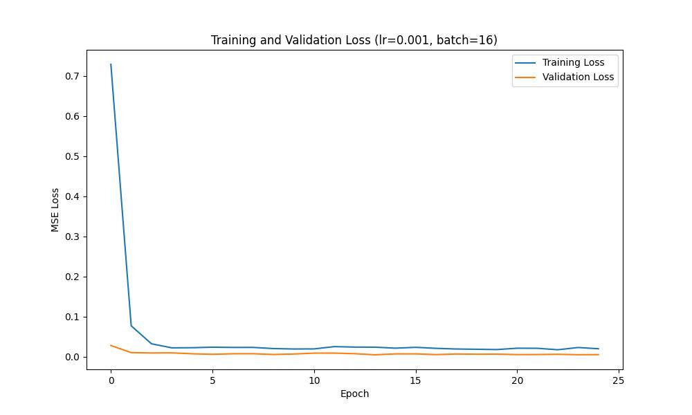
We can plot the training and validation loss curves across each epoch to show the training progress; such curves are shown below:
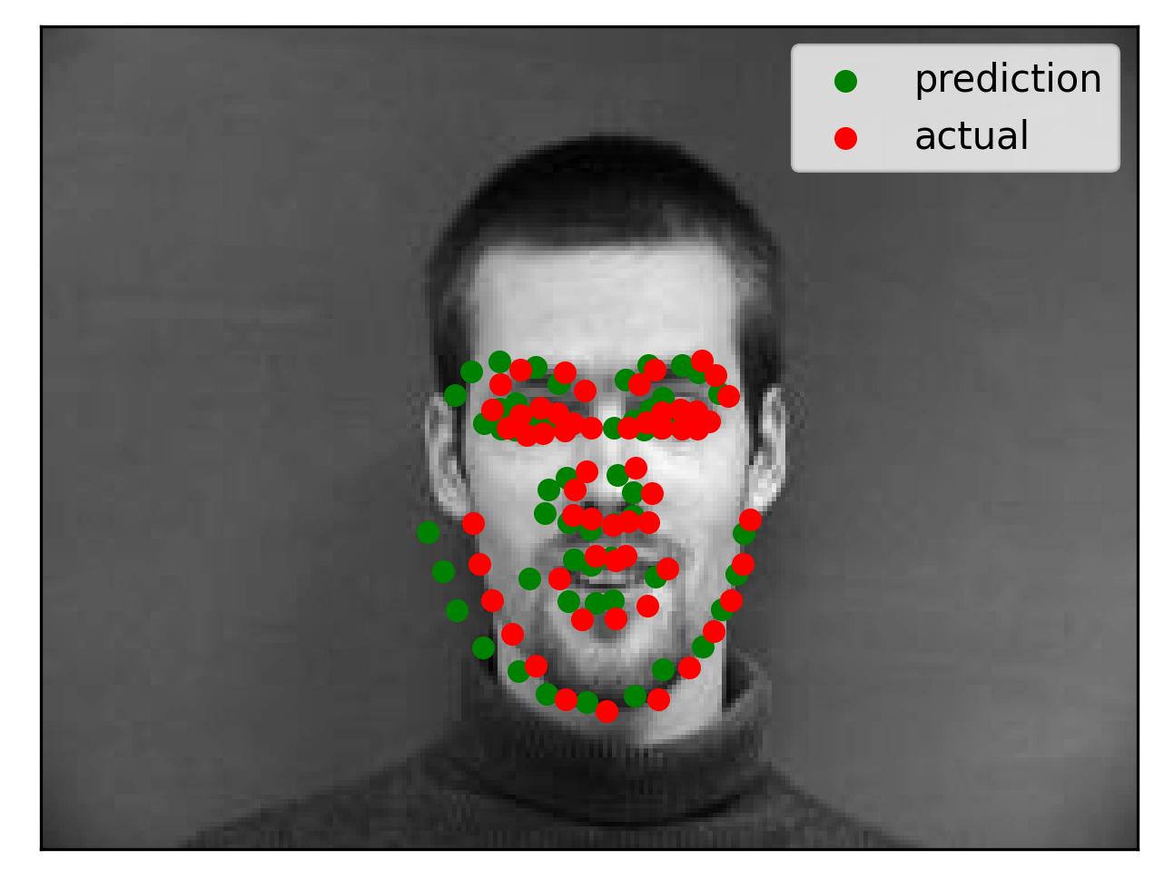
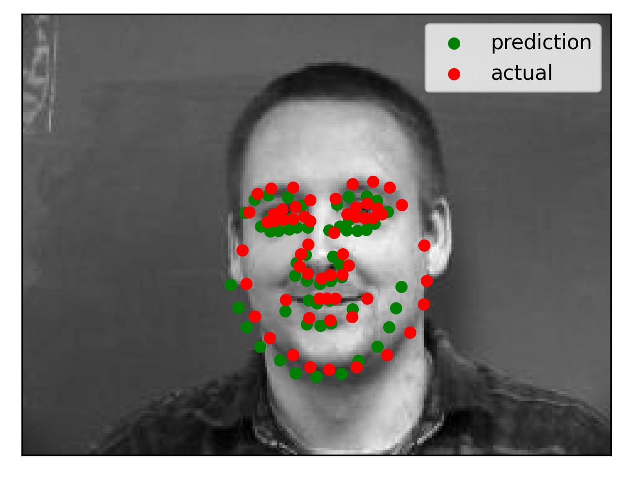
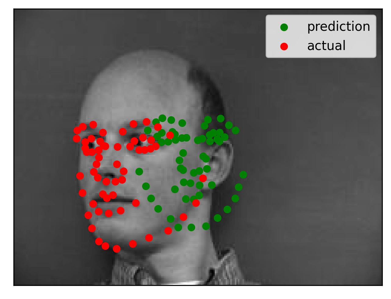
While my model performed well, there were examples in which it did not work well. Shown below are two failure cases and two successful cases.
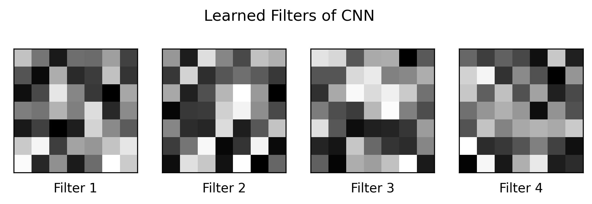
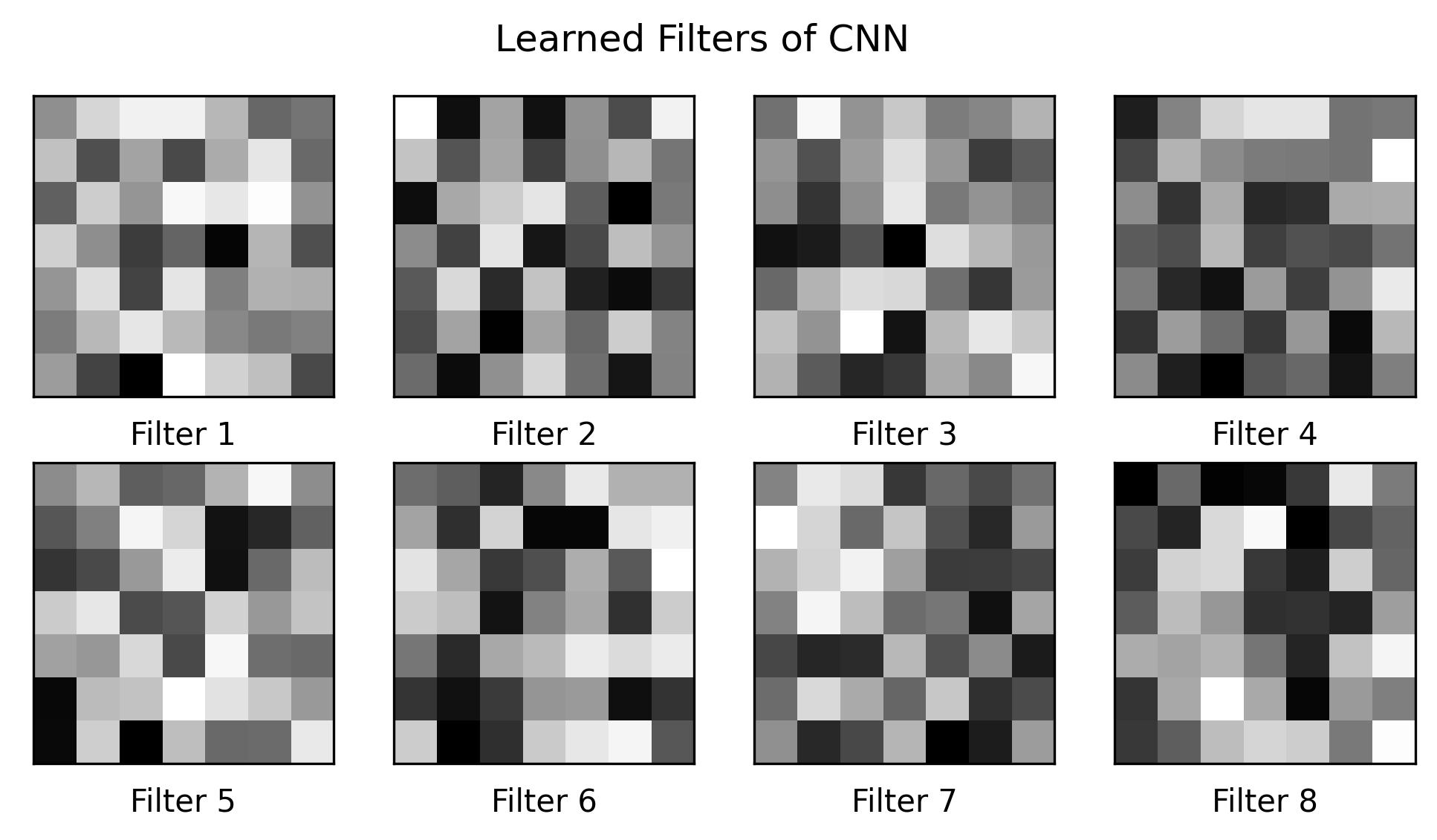
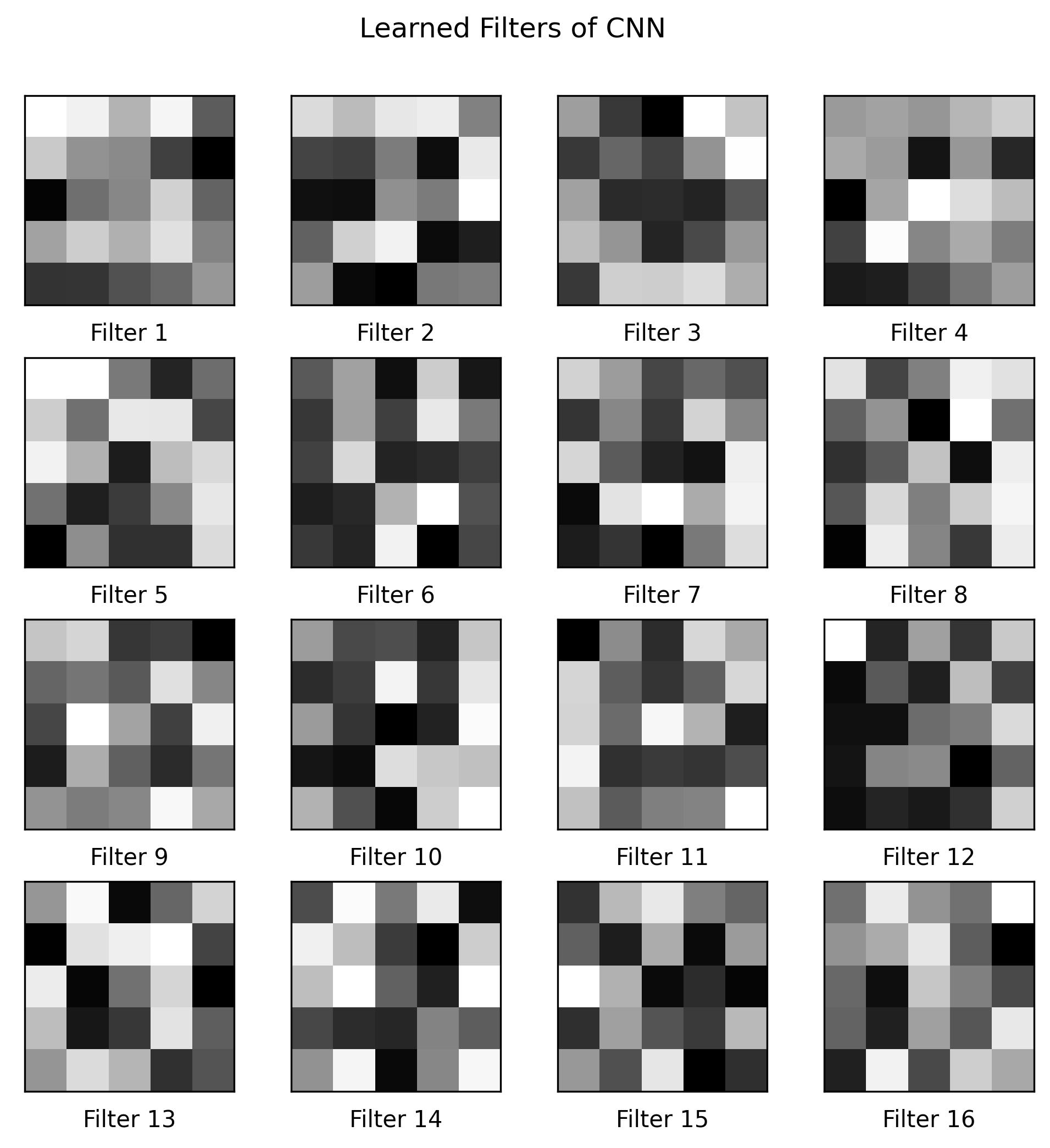
We can visualize the filters that the CNN learned along training time by looking at the model's weights. The first two convolutional layers have (7,7) kernels, while convolutional layers 3-5 have kernels of size (5,5). To visualize such filters, I needed to sift through the model and its attributes, locating the learned weights in the process; some of the weights are shown below:
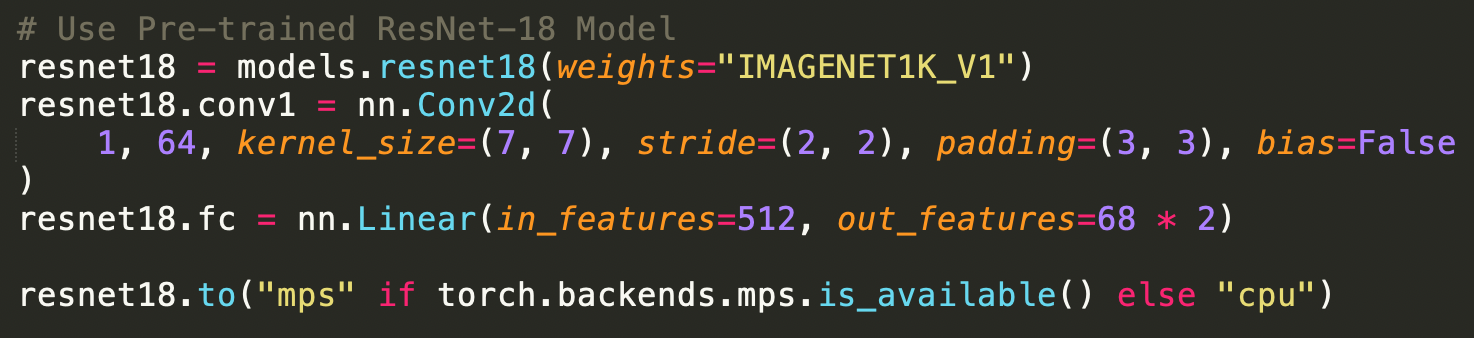
For this part, we used a larger dataset, specifically the IBUG face in the wild dataset for training a facial keypoints detector. This dataset contains 6666 images of varying image sizes, and each image has 68 annotated facial keypoints. To train the model, I used the pretrained ResNet-18 model provided by Pytorch, modifying the first convolutional layer to accept a grayscale image with one image channel and modifying the last linear layer to return the 136 keypoint coordinates. I trained the model using a learning rate of 0.001 for 20 epochs and the MSE loss function. I used the MPS Pytorch Backend to take advantage of the M1 Chip's Optimized training.
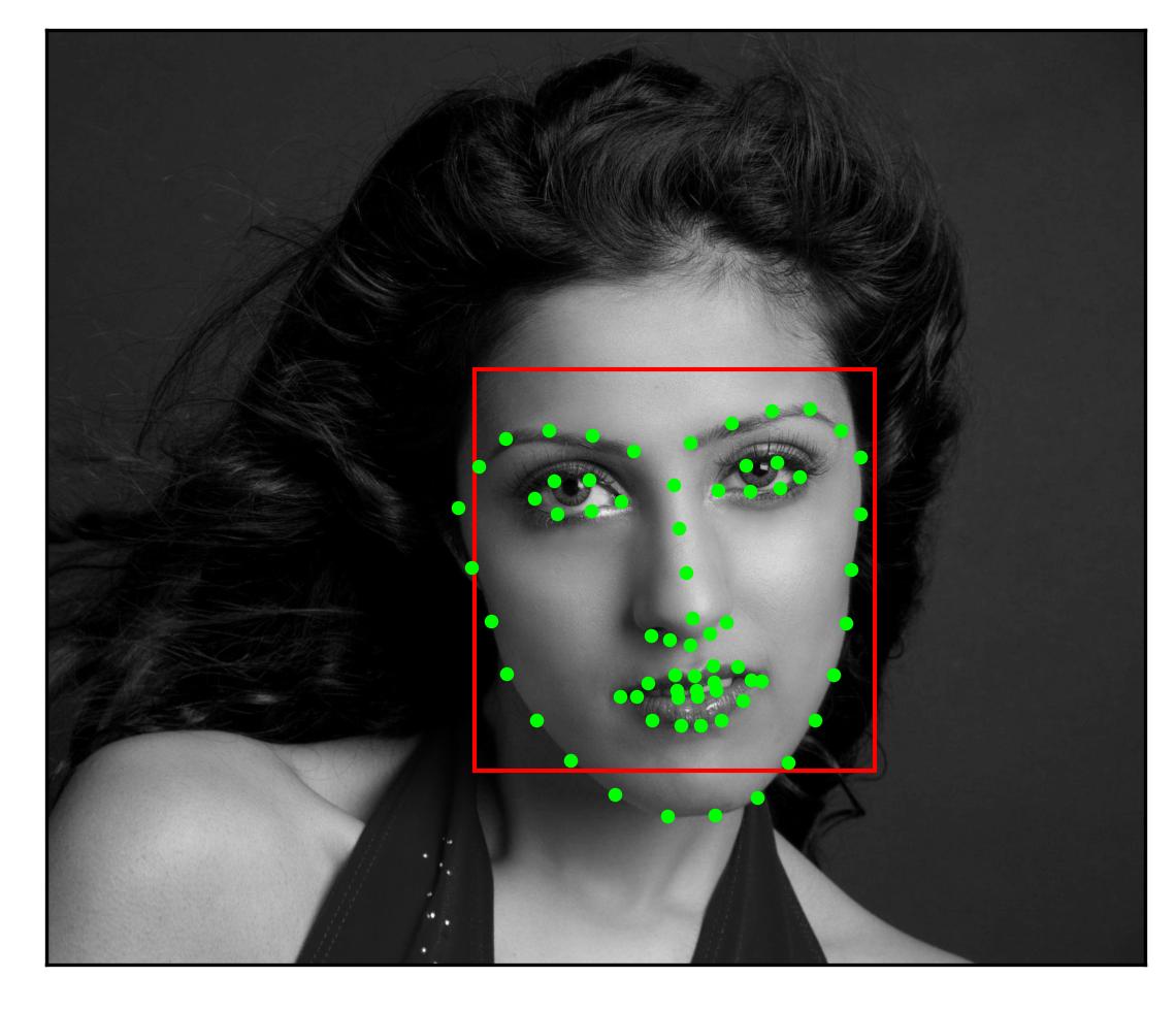
Each image in the IBUG Dataset comes with its facial keypoints and a corresponding bounding box. I standardized each image by first cropping the image to only include the area within the bounding box and resizing to (224, 224). A sample image is shown below with its bounding box and keypoints.
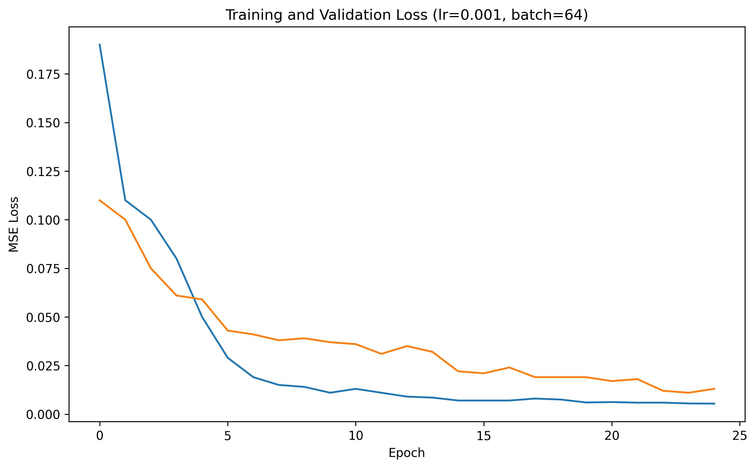
We can plot the training and validation loss curves across each epoch to show the training progress; such curves are shown below:
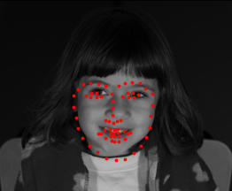
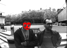
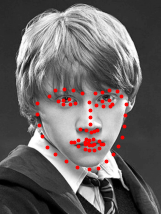
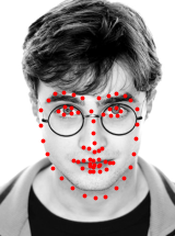
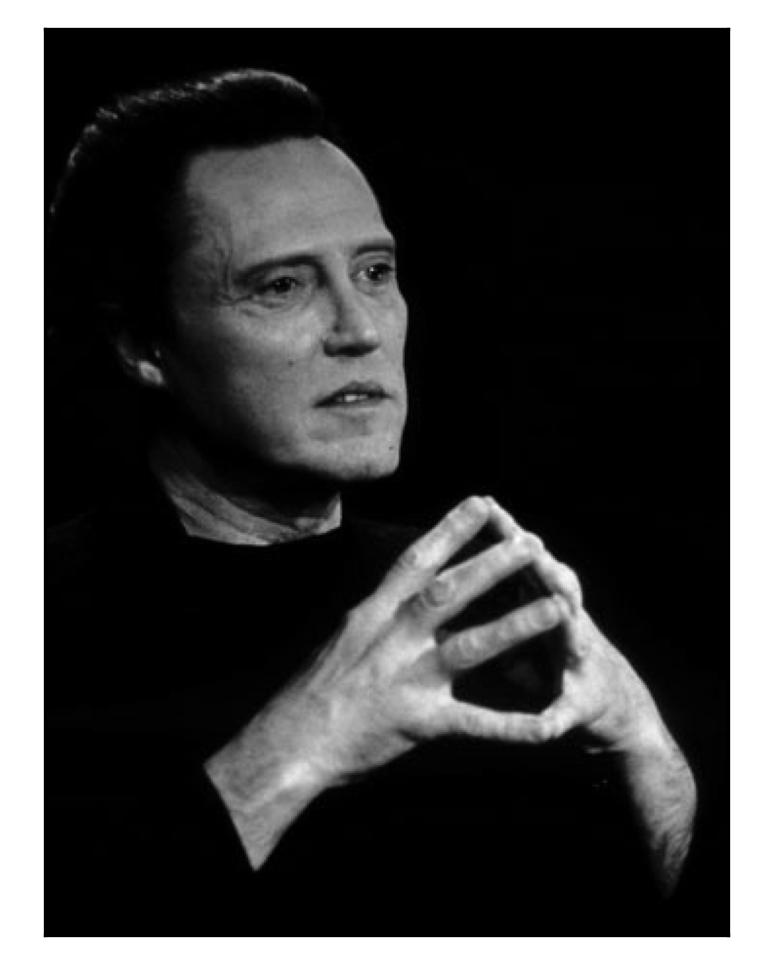
We can run our trained model on some images from the test set. The results are shown below. My model does a solid job at identifying the facial structure of a person within the image. When there are multiple people within an image, it only finds one.

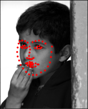
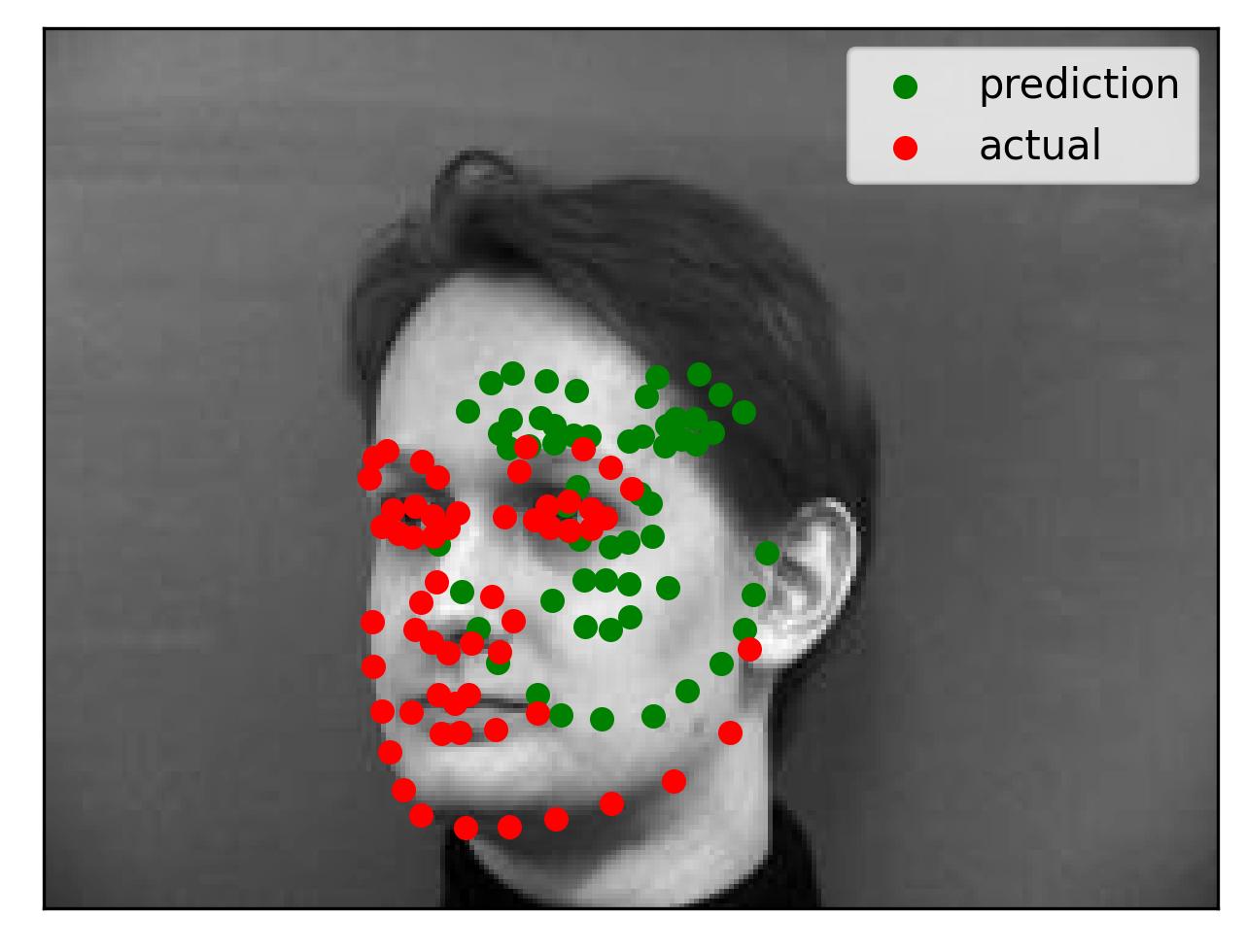
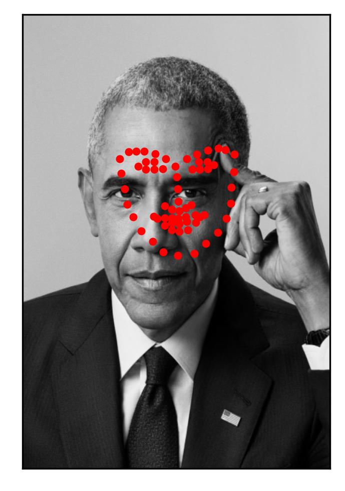
We can also run the model on several images of my own to show the power of the trained model. While it works in many cases, it fails from time to time (as shown below):
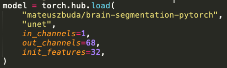
More keypoint detection networks such as Toshev et. al. (2014) or Jain et. al. (2014) turn the regression problem of predicting the keypoint coordinates into a pixelwise classification problem: for every pixel, they predict how likely is that pixel is the keypoint? I used the U-Net architecture to predict keypoints using a classification-based approach. I used a pre-exisitng U-Net architecture that was modified to take in a greyscale image (one channel) and output a (68, 224, 224) tensor where each channel represented the output for a given facial keypoint. The architecture is shown below:
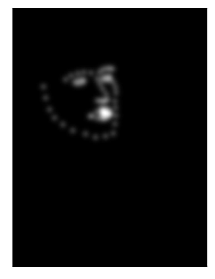
To turn this into a classification problem, I turned my ground truth keypoint coordinates into pixel-aligned heatmaps to supervise my model by placing 2D Gaussians at the ground truth coordinate location in the map. A few sample images and their corresponding 2D Gaussians are shown below. Each ground-truth keypoint had a corresponding Bivariate Gaussian distribution with a mean vector of (x,y) (i.e. that ground-truth keypoint) and a covariance matrix of [[25, 0], [0, 25]]. I found that a variance of 25 was enough to generalize the keypoint enough but not high enough where the mask became a jumble of keypoints. I stacked all heatmaps onto each other to produce a single visual.


Unfortunately I did not have time to train this portion of the project. In my efforts, both the training and validation losses never seemed to go down. I found that this part of the project also took significantly longer to train, thus I don't have results to show.
The mean absolute error (MAE) for my best performing model was 24.21591. You can find the submission on Kaggle here. My Kaggle username is "Will Furtado".This model used the pre-trained ResNet-18 as a base, a learning rate of 0.001 trained on 20 epochs using Pytorch accelerated by the M1 Chip (MPS Backend). It used the Adam optimizer. This model is the same as presented in Part 3 on the project.