As this paper by Ng et al. (Ren Ng is the founder of the Lytro camera and a Professor at Berkeley!) demonstrated, capturing multiple images over a plane orthogonal to the optical axis enables achieving complex effects using very simple operations like shifting and averaging. The goal of this project is to reproduce some of these effects using real lightfield data, namely depth refocusing and aperature adjustment.
When working with lightfield camera images, the objects which are far away from the camera do not vary their position significantly when the camera moves around while keeping the optical axis direction unchanged. The nearby objects, on the other hand, vary their position significantly across images. Averaging all the images in the grid without any shifting will produce an image which is sharp around the far-away objects but blurry around the nearby ones. Similarly, shifting the images 'appropriately' and then averaging allows one to focus on object at different depths. For the depth refocusing aspect of the project, I generate multiple images, each which focus at different depths based on the series of input images. To do so, I use the following approach as described in the paper above:
            center (U, V) <- find center image based on center (X,Y)

            for each image:
                shift <- displacement from center (U, V) to image (U, V)
                shifted image <- multiply each shift by alpha and shift original image

            average all shifted images
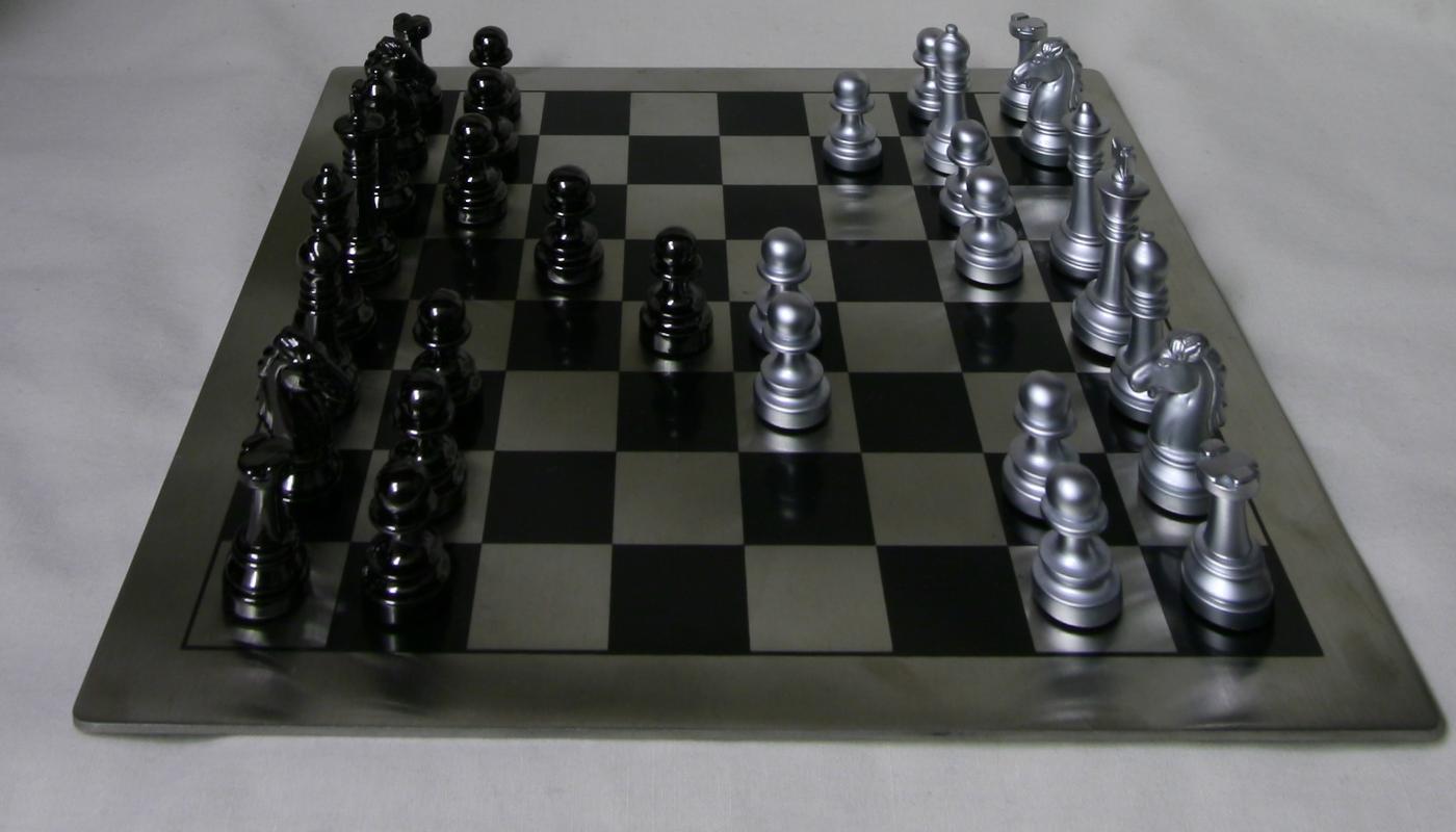
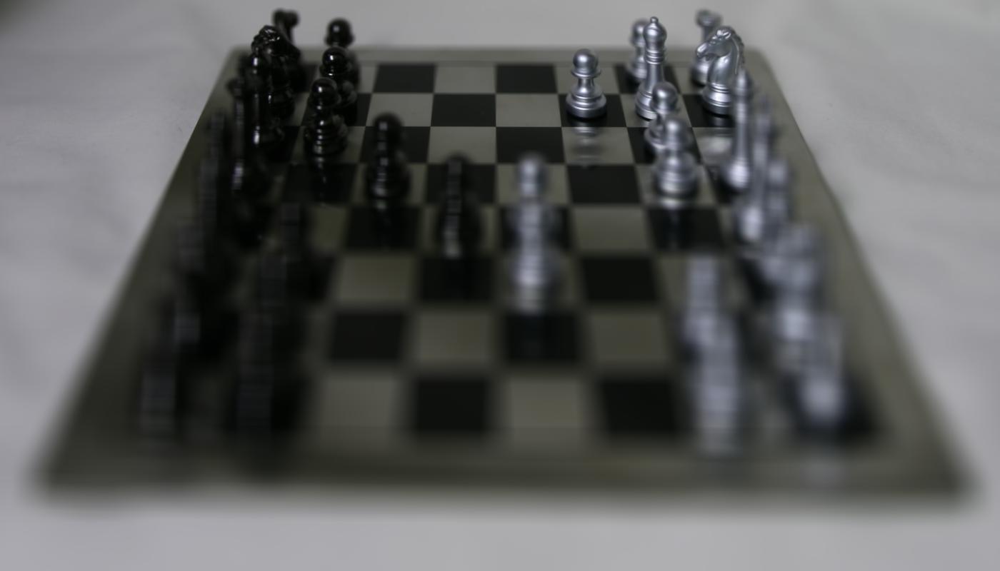
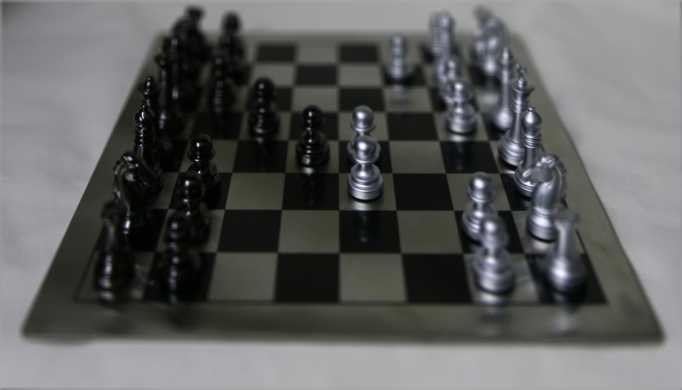
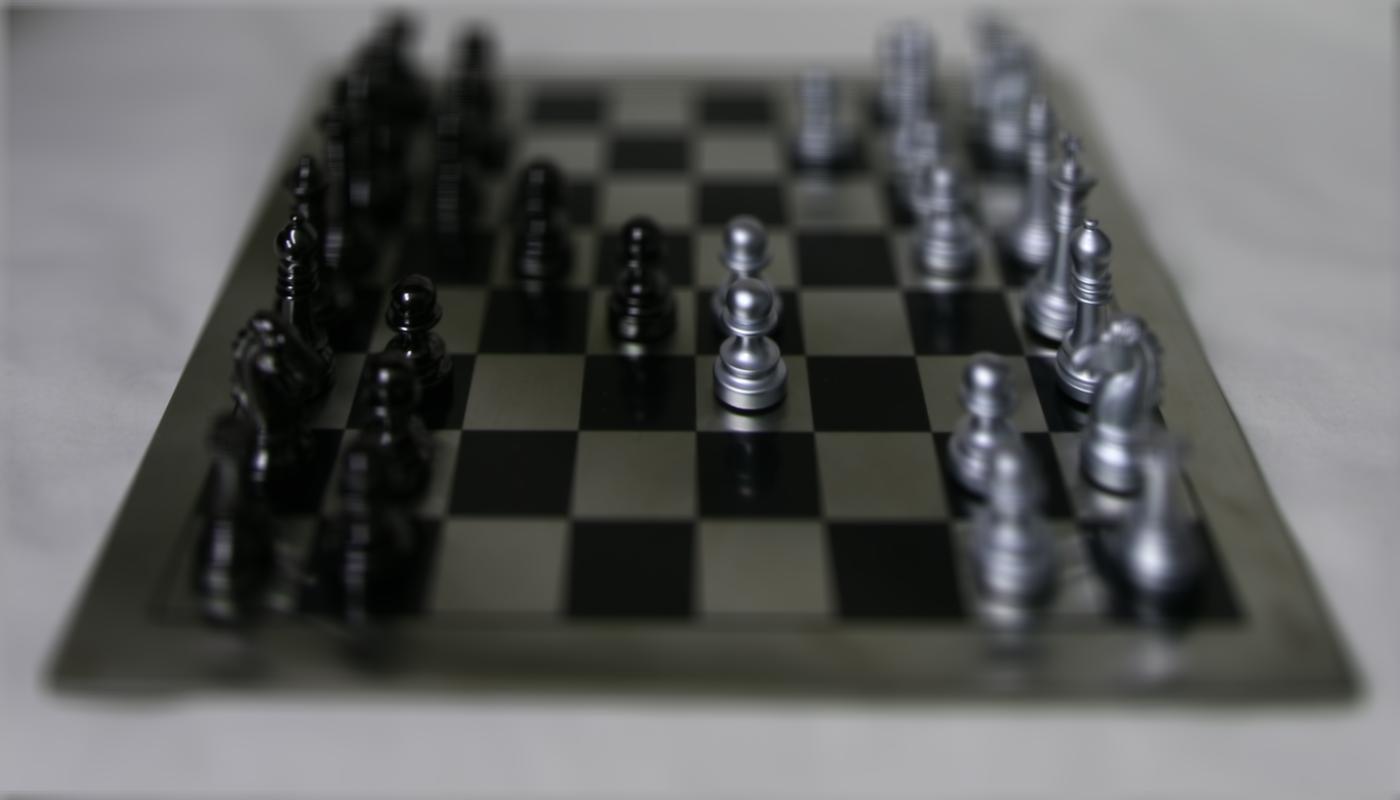
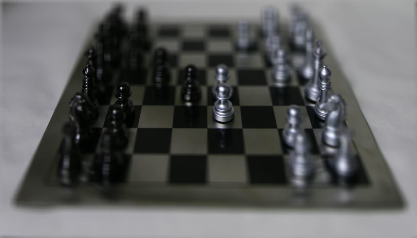
Below I've shown one such image example at a fixed depth and the result of naively averaging all images together with no shifting. As described above, a simple average results in the close-up parts of the image being blurry.
I've also shown the simulation of a camera focusing at different depths by creating a GIF that loops through various values of the refocusing hyperparameter α within the range -0.8 to 0.8 (step size of 0.1). The focus shifts from the top right corner of the image, through the middle, ending in the bottom left corner.
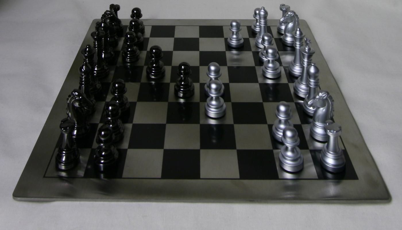
Averaging over a large number of images sampled over the grid perpendicular to the optical axis mimics a camera with a much larger aperture. Similarly, using fewer images results in a smaller aperture. For this part of the project, I simulated both small and large apertures using the set of chess images.
To do so, I fixed the refocusing hyperparameter to -0.3 so that we could visually distinguish between different aperture levels. This parameter was best for viewing the center of image in the most clear view. The smallest possible aperture would only focus on a single image, while the largest possible aperture would average all images together. To simulate aperture, I introduce a new hyperparameter, radius, which sets a criterion for which images to include in the final averaging; only images that are of distance less than radius will be included.
Below I've shown a series of photos simulating small to large apertures as achieved by the technique above.


I've also shown the simulation of a camera adjusting at different apertures by creating a GIF that loops through various values of the hyperparameter radius; within the range 1 to 10 (step size of 1). The focus gets wider as the aperture decreases (i.e. radius decreases).
radius between [1, 10] with step size of 1In this project, I learned that we can simulate both a camera's depth of field and aperture using only image processing and computer vision techniques. Previously, I thought there was no way to recover these sorts of transformations on images.
In this augmented reality project, I captured a video using my iPhone and inserted a synthetic object into the scene I recorded. Simply put, the key task for this project was to use 2D points in the image whose 3D coordinates are known to calibrate the camera for every video frame and then use the camera projection matrix to project the 3D coordinates of a cube onto the image. If I calibrated the camera correctly, the cube should appear to be consistently added to each frame of the video. The original video is shown below.
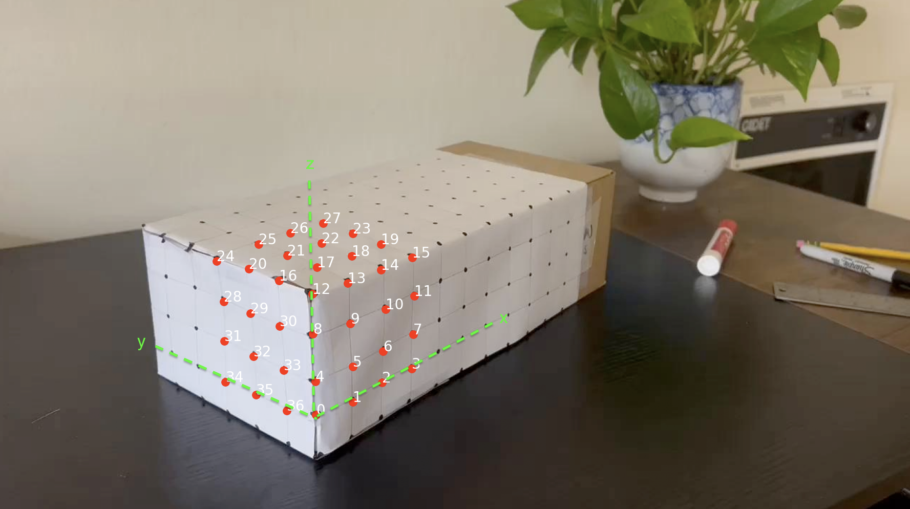
In order to calibrate the camera for each frame, I needed to create my own three-dimensional grid using a shoebox and a ruler. I labeled three-dimensional points on the shoebox by creating a grid of one inch by one inch boxes. I used a ruler and pencil, making note to be as precise as possible, as the more exact the grid was, the more effective the projection would be. I ended up using 37 reference points to form a nice cube. I chose the bottom corner (as shown below) to be the origin, (0,0,0), in the 3D coordinate space. Each axis is labeled.
In order to track the reference points throughout the video, we need a method to propogate the points from the starting frame to the subsequent frames. I used OpenCV's CSRT (Discriminative Correlation Filter with Channel and Spatial Reliability) Tracker from cv2.legacy with a patch size of (8 x 8) to obtain the smoothest and most reliable tracking results. Originally, I used the suggested MedianFlow tracker but found that the bounding boxes exploded in size as the video progressed. The results of the point tracking are shown below:
The calibration of the camera resulted in the 2D image coordinates of marked points and their corresponding 3D coordinates. I then used these coordinates and least squares to fit the camera projection matrix to project the four-dimensional real world coordinates to three-dimensional image coordinates (both homogeneous coordinates). For each frame in the video, I repeated this process to obtain its unique projection matrix.
Once I computed the camera projection matrix for each frame, I projected the corners of the cube (defined using the 3D-coordinate grid) and used the draw function that was provided to draw the cube on the image. The results are shown below, both with and without the reference bounding boxes. I'm quite happy with the results.
The augmented reality project taught me more than I ever thought I could conquer in the world of AR. Hopefully I can use these skills to get a job with Niantic working on Pokemon Go!