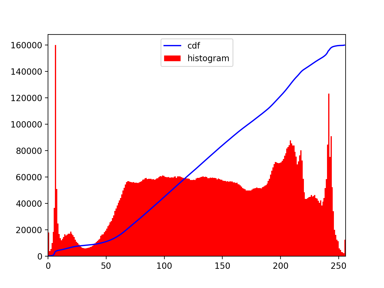
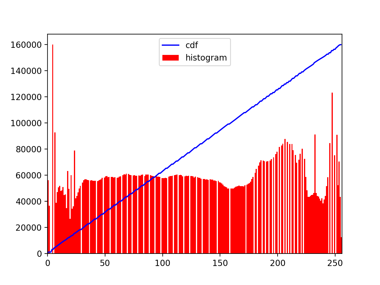
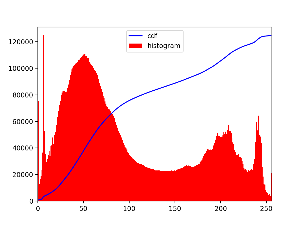
icon.tif pixel value distributions of B, G, R channel (original)

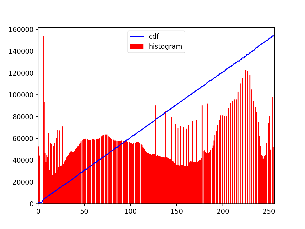
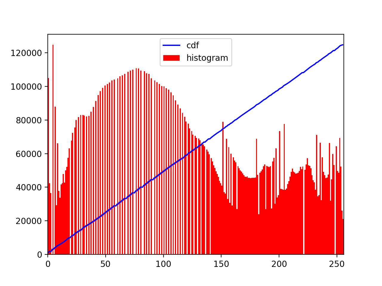
icon.tif pixel value distributions of B, G, R channel (after histogram equalization)


Automatic Contrasting [Bells and Whistles]
I use histogram equalization for contrast adjustment. For each color channel with pixel values ranging from 0 to 255, create a histogram of pixel value. Compute the cumulative distribution function for the histogram and normalize the cdf. Find the new pixel values given the normalized cdf.

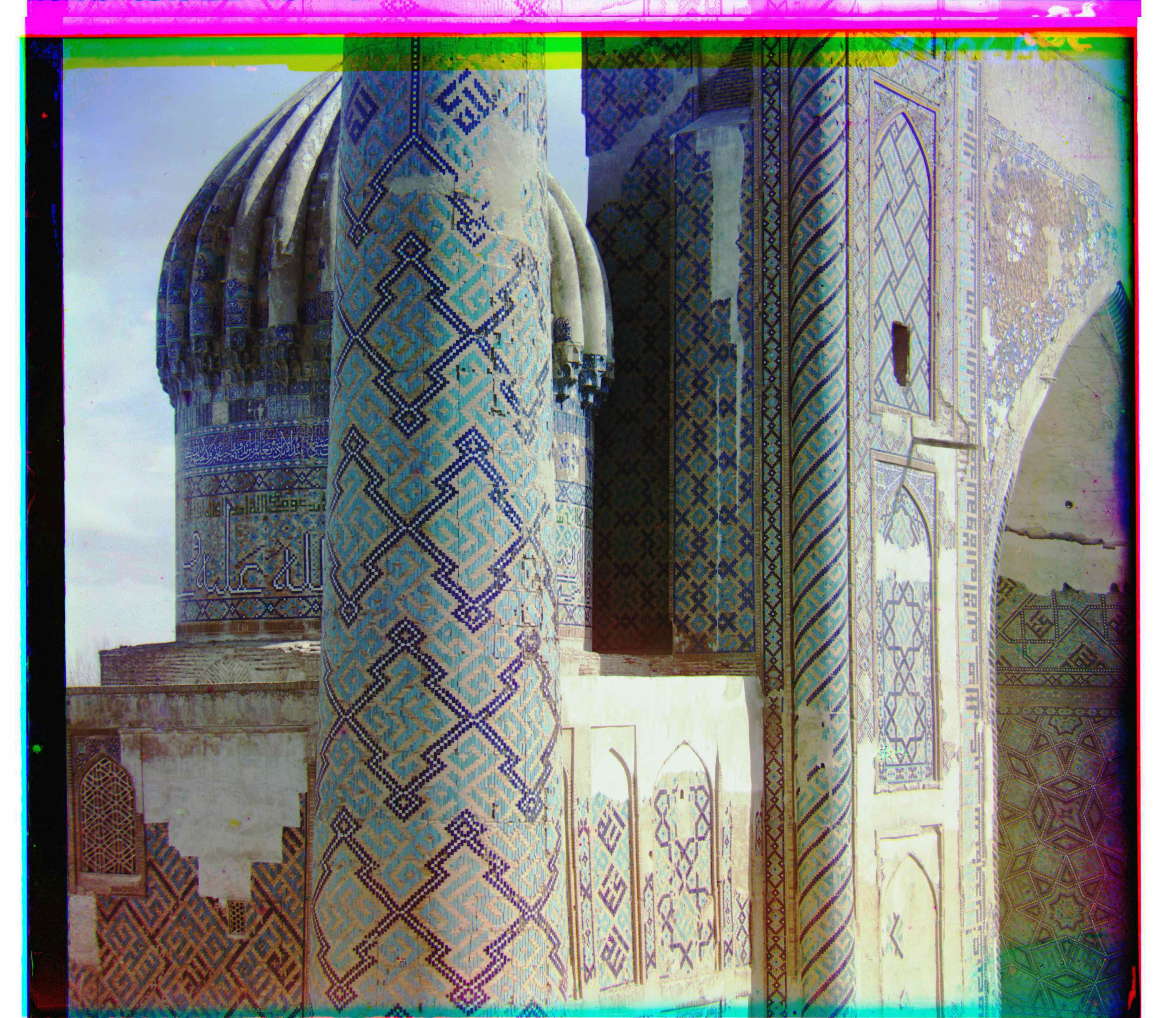
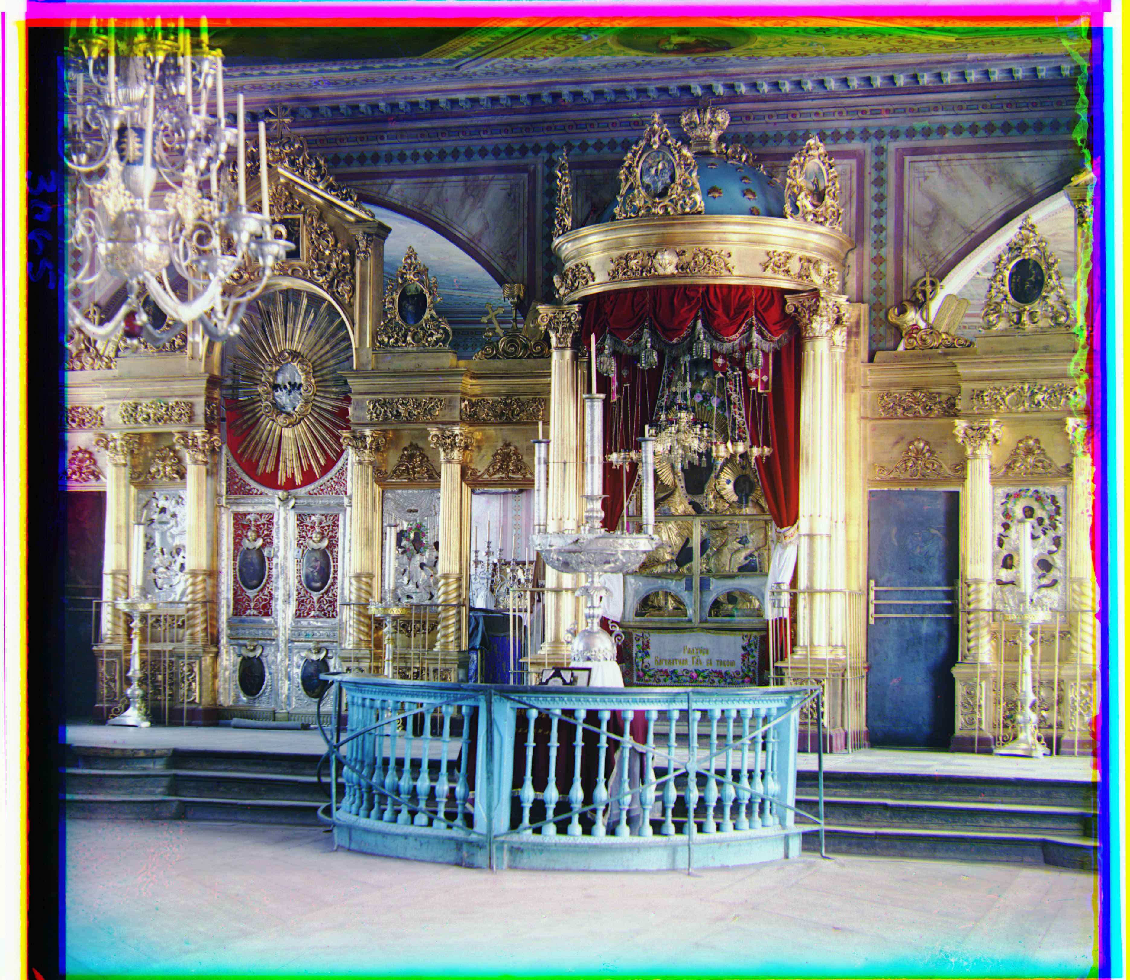
icon.tif (before contrasting)

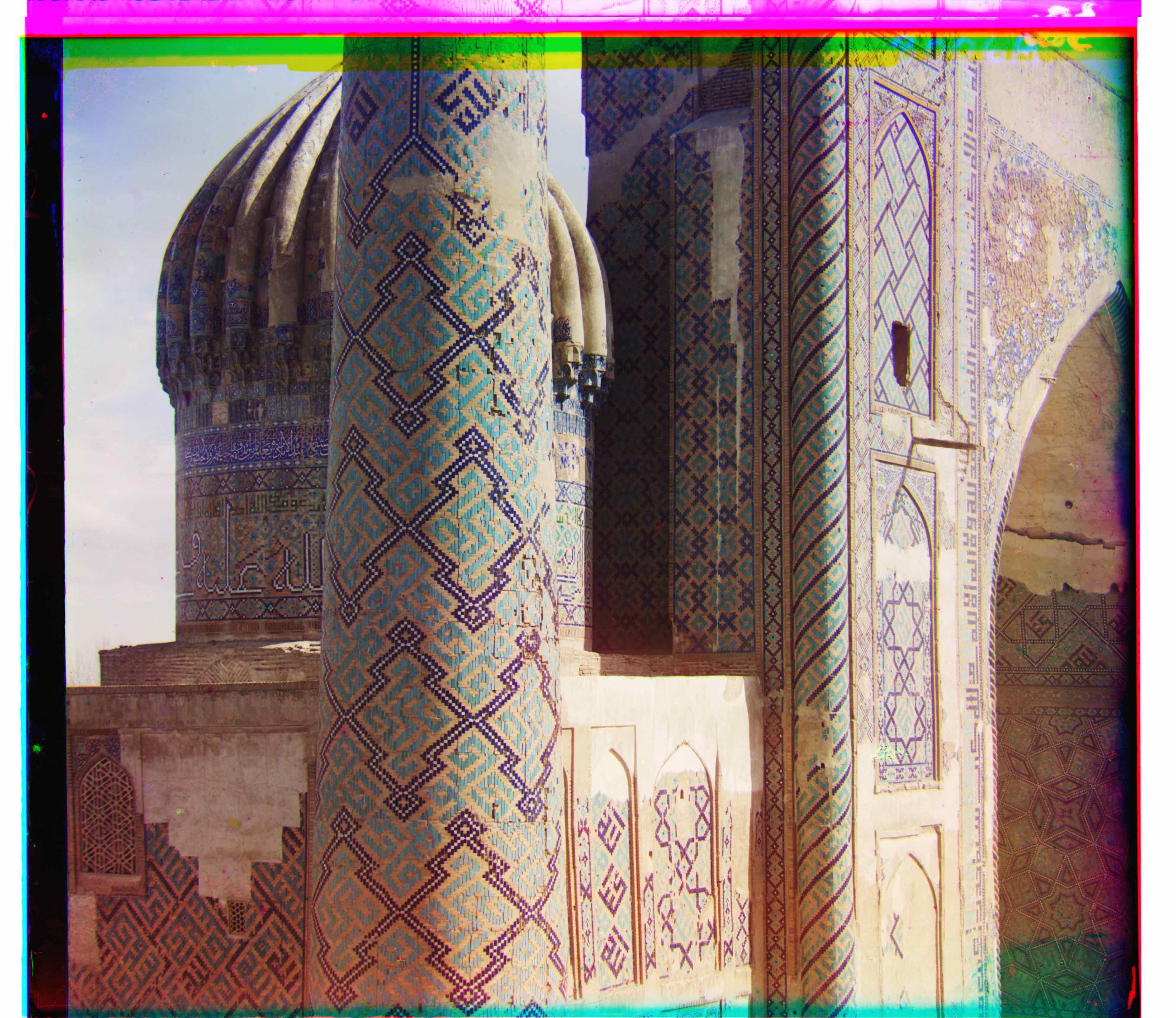
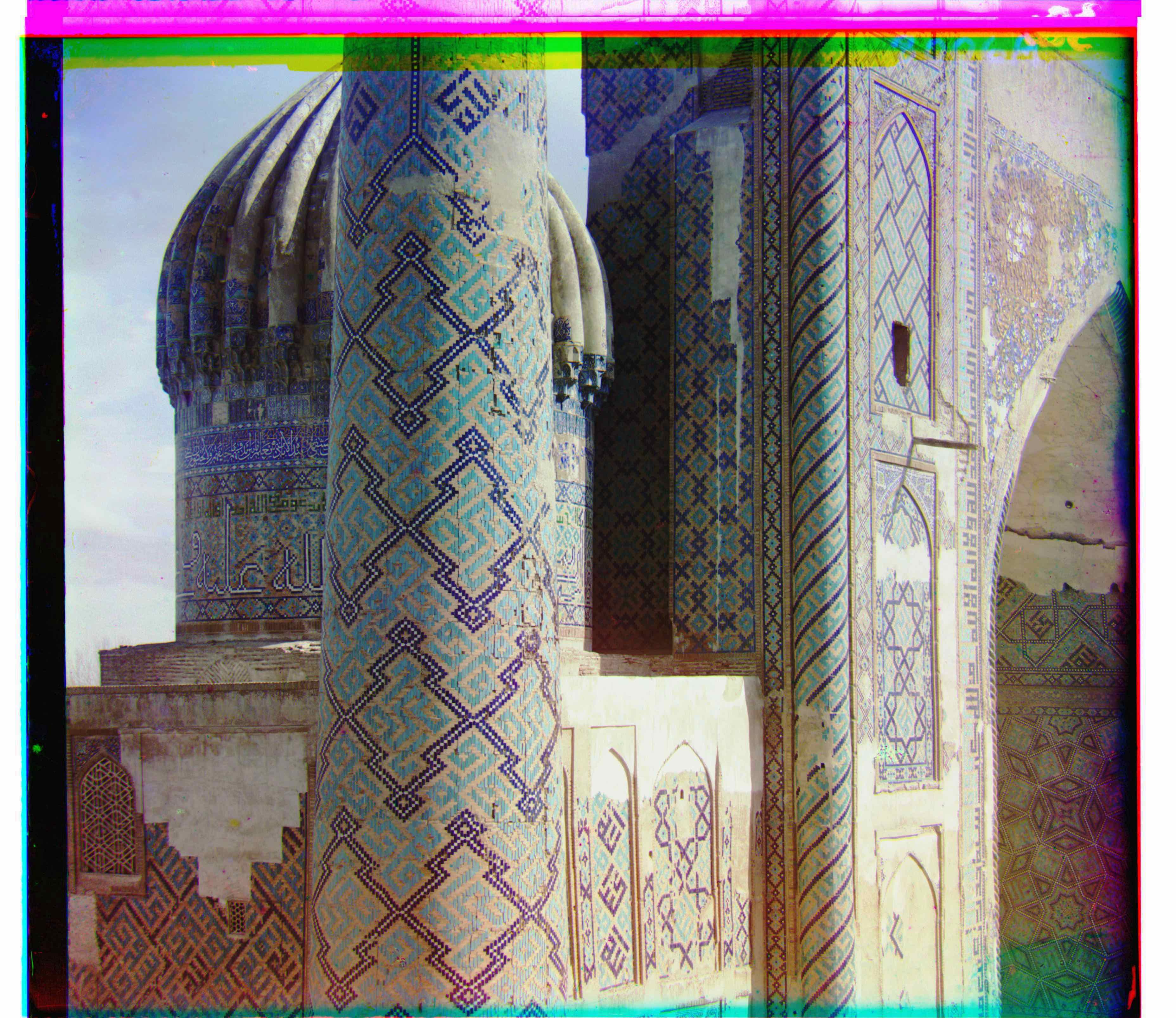
icon.tif (after contrasting)

g: (40, 17); r: (89, 23)

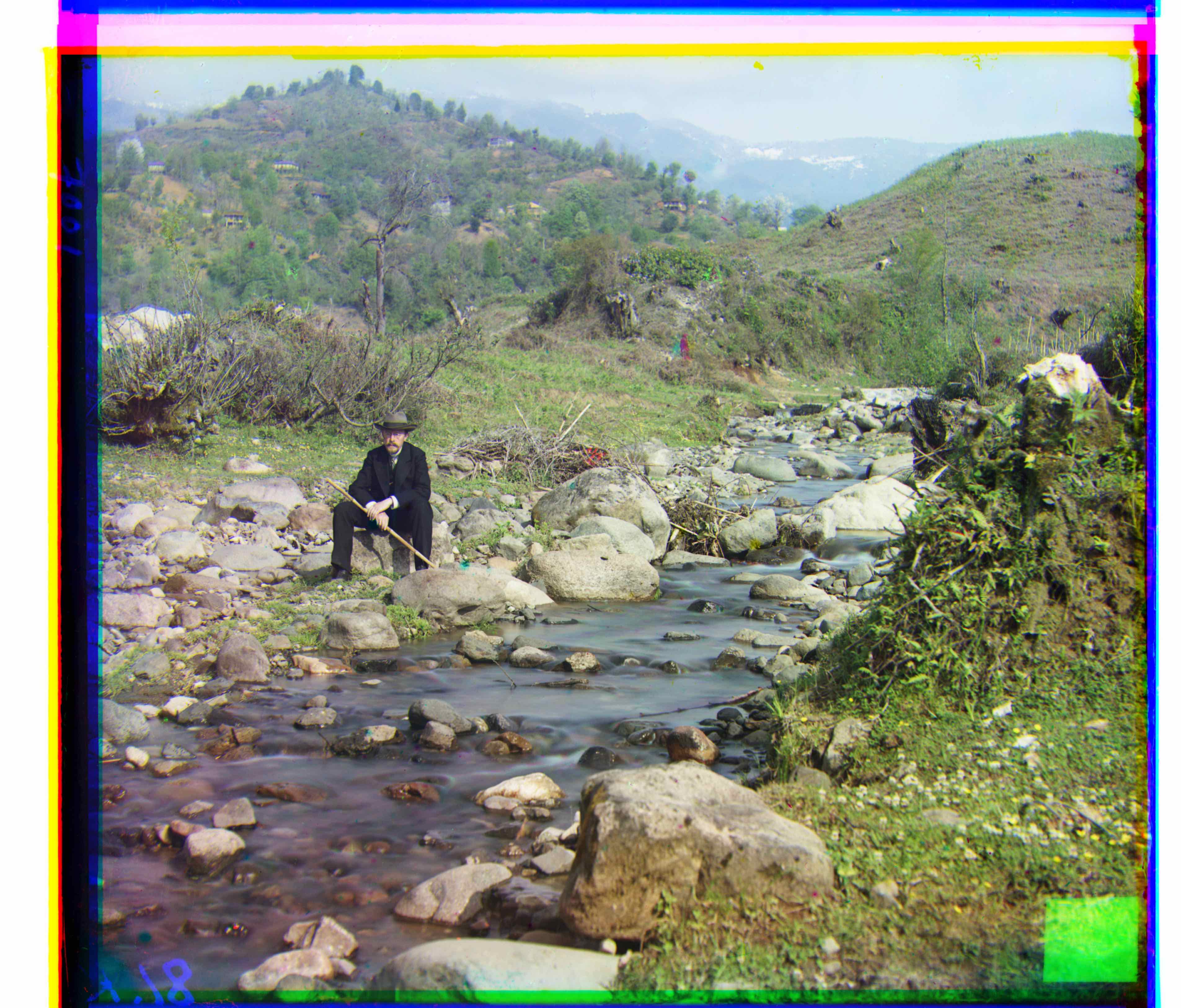
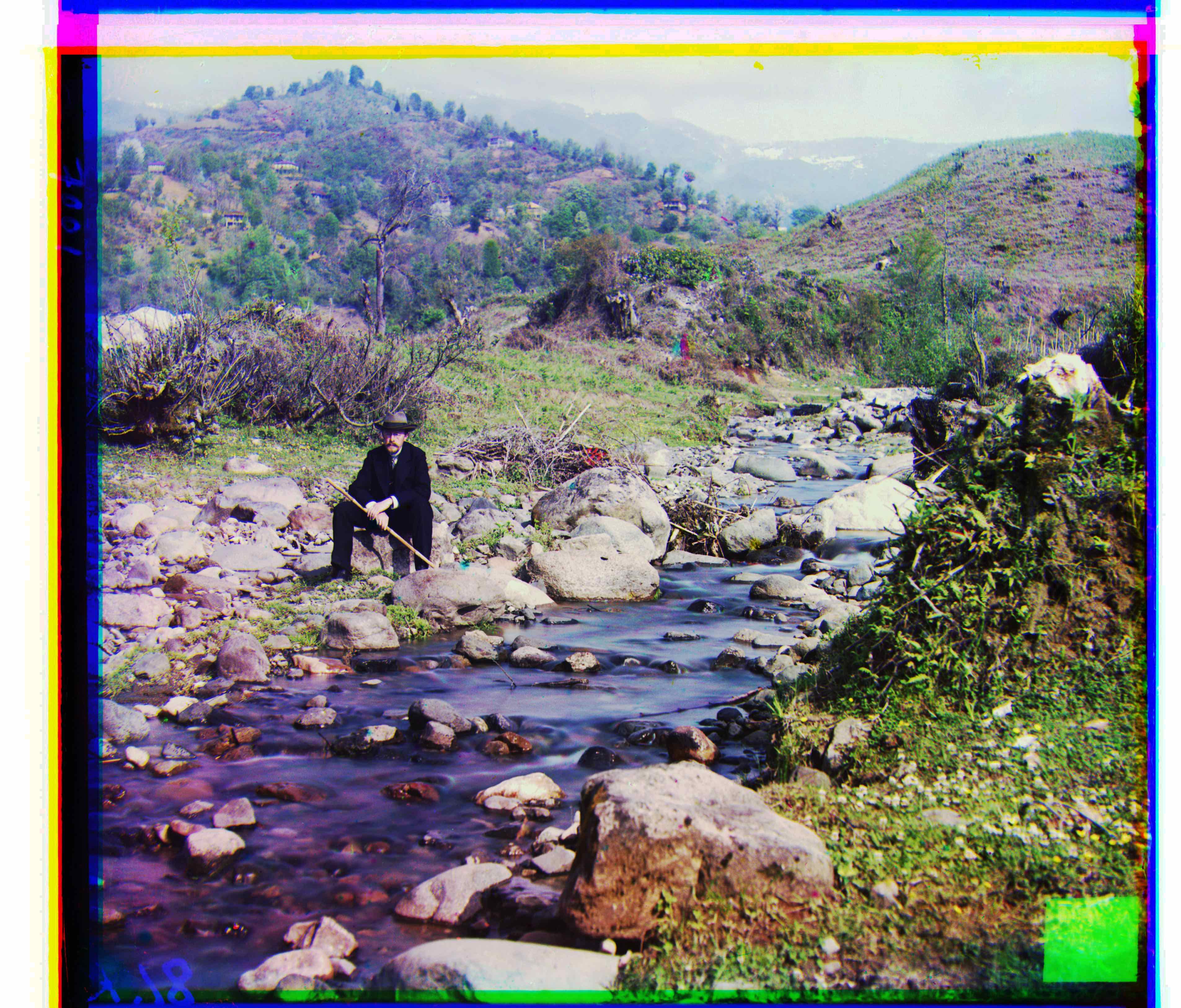
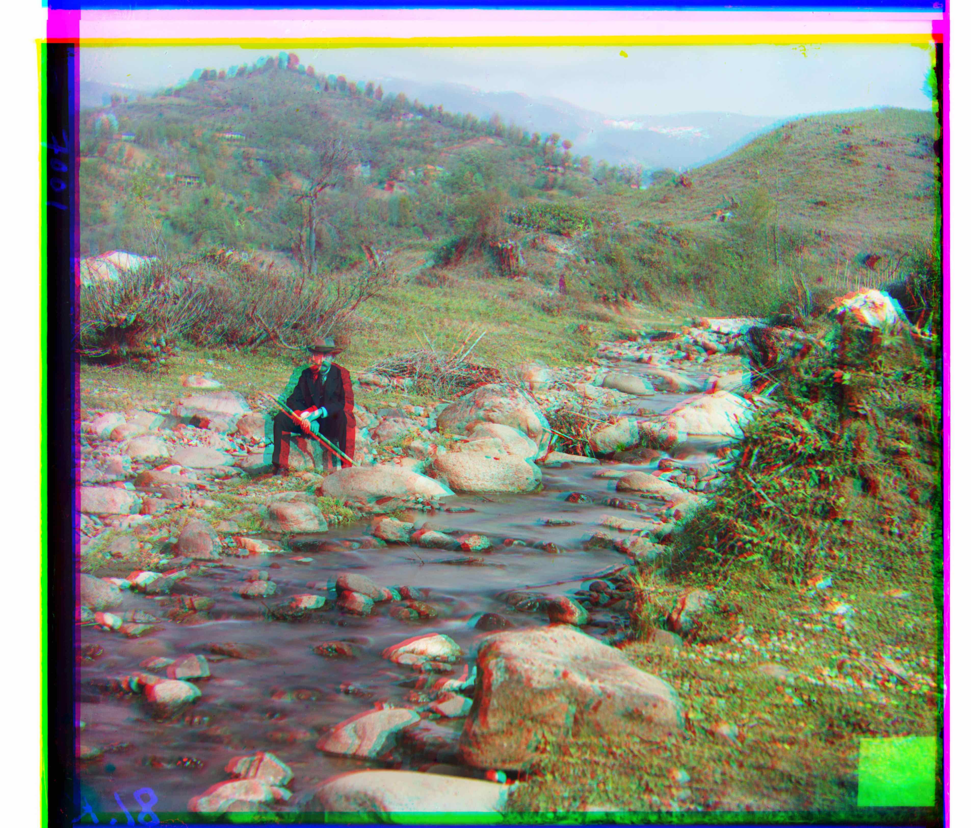
self_portrait.tif (before contrasting)
self_portrait.tif (after contrasting)
g: (40, 17); r: (89, 23)
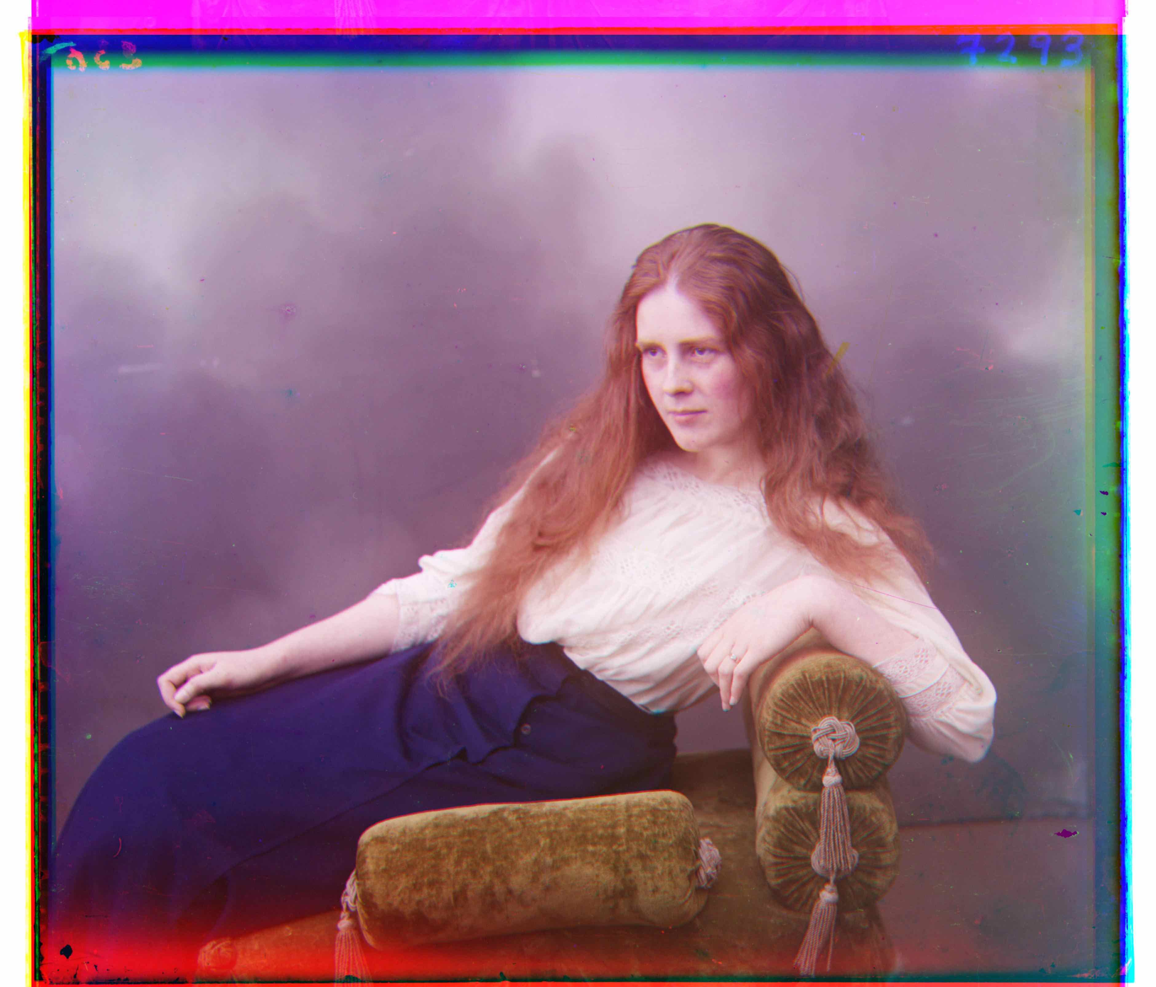
lady.tif (before contrasting)
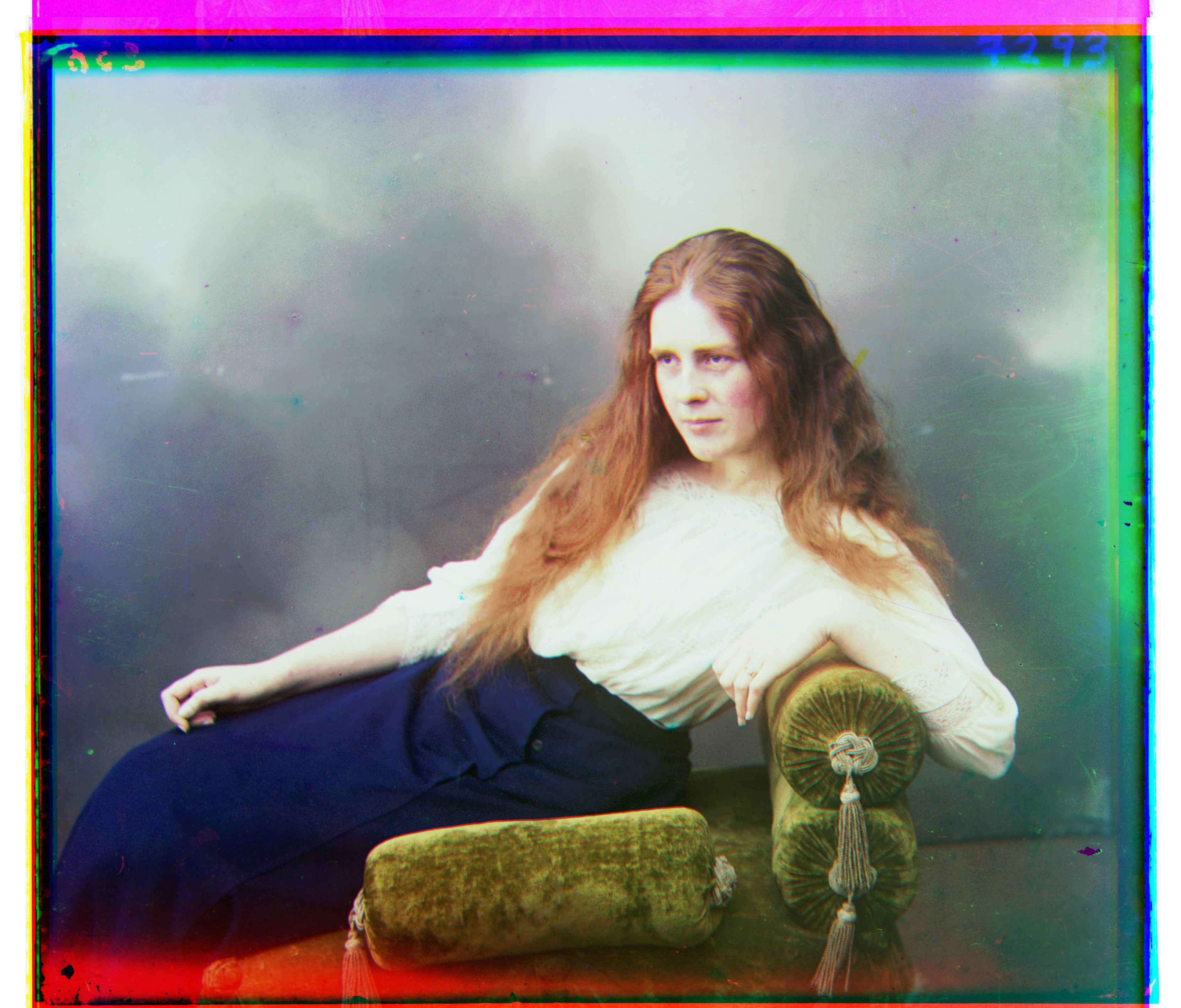
lady.tif (after contrasting)
g: (55, 8); r: (113, 9)
Project 1: Colorizing the Prokudin-Gorskii Photo Collection
CS194-26: Image Manipulation and Computational Photography

Overview
In early 20th century, a Russian man named Sergei Mikhailovich Prokudin-Gorskii envisioned a plan to document the vast Russian Empire using new advancements in color photography. He traveled across the country and took thousands of pictures of people, buildings, landscapes... For each scene, he recorded three exposures onto a glass plane using a red, a green, and a blue filter. These valuable glass plates were later purchased by the Library of Congress. The LoC digitized the negatives and made them public on-line.
In this project, I utilize image processing techniques to automatically produce color images from the digitized Prokudin-Gorskii glass plate images. The program extracts the three color channel images from a glass plate image and aligns them to form a single RGB color image.
Approach
The original glass plate image is divided vertically into three equal parts, corresponding to B, G, R channels. To align two parts, search within a window of possible displacements and choose the displacement with the best score using some metric described below. Because the edges of the three channels cannot be aligned anyway and create noise, I disregard 5% area of each edge when computing losses.
Metrics to measure the quality of alignment:
- L2 loss: sum of squared differences between two images
- NCC loss: the negative of the dot product between two normalized images
For low resolution images (~300*300 pixels), I search in range [-15, 15] pixels along each axis. Using two metrics renders identical result for every image. For high resolution images (~3000*3000 pixels), an exhaustive search over a reasonable range of displacement is too slow. Therefore, I use a coarse-to-fine image pyramid to search for the correct displacement. The image is downscaled by a factor of 2 at a coarser level. The image is first aligned at the coarsest level (smallest scale), then at a finer level, a search in range [-1, 1] pixel along each axis is sufficient to find the best adjustment to the previous estimate of the correct displacement. While using two metrics achieves similar results for most images, NCC loss performs obviously better on some images such as emir.tif and self_portrait.tif.
self_portrait.tif using L2 loss self_portrait.tif using NCC loss
Results on Low-Resolution Images

cathedral.jpg
monastery.jpg
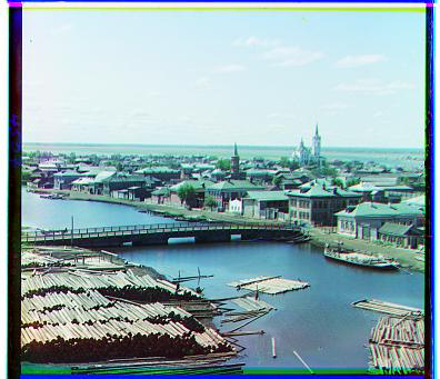
tobolsk.jpg
g: (5, 2); r: (12, 3)
g: (-3, 2); r: (3, 2)
g: (3, 2); r: (6, 3)
Results on High-Resolution Images (use NCC loss)
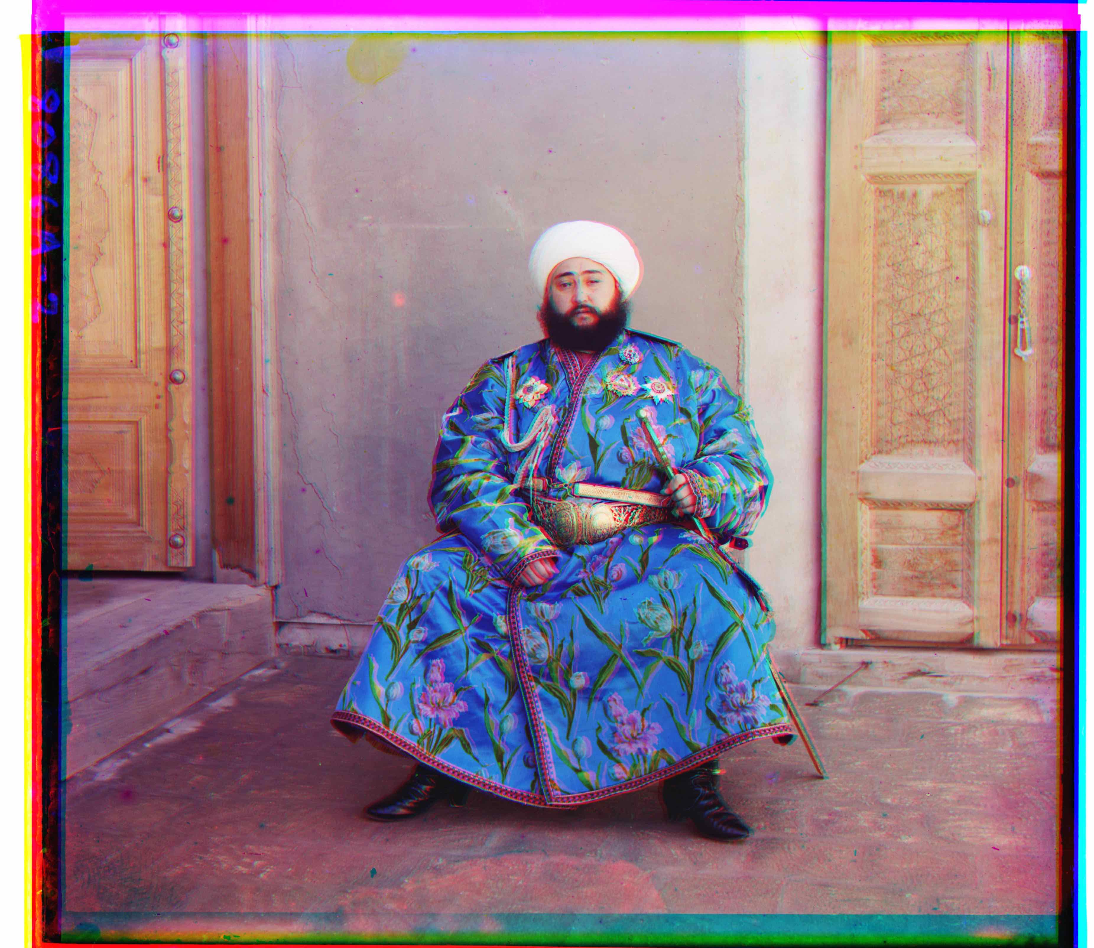
emir.tif
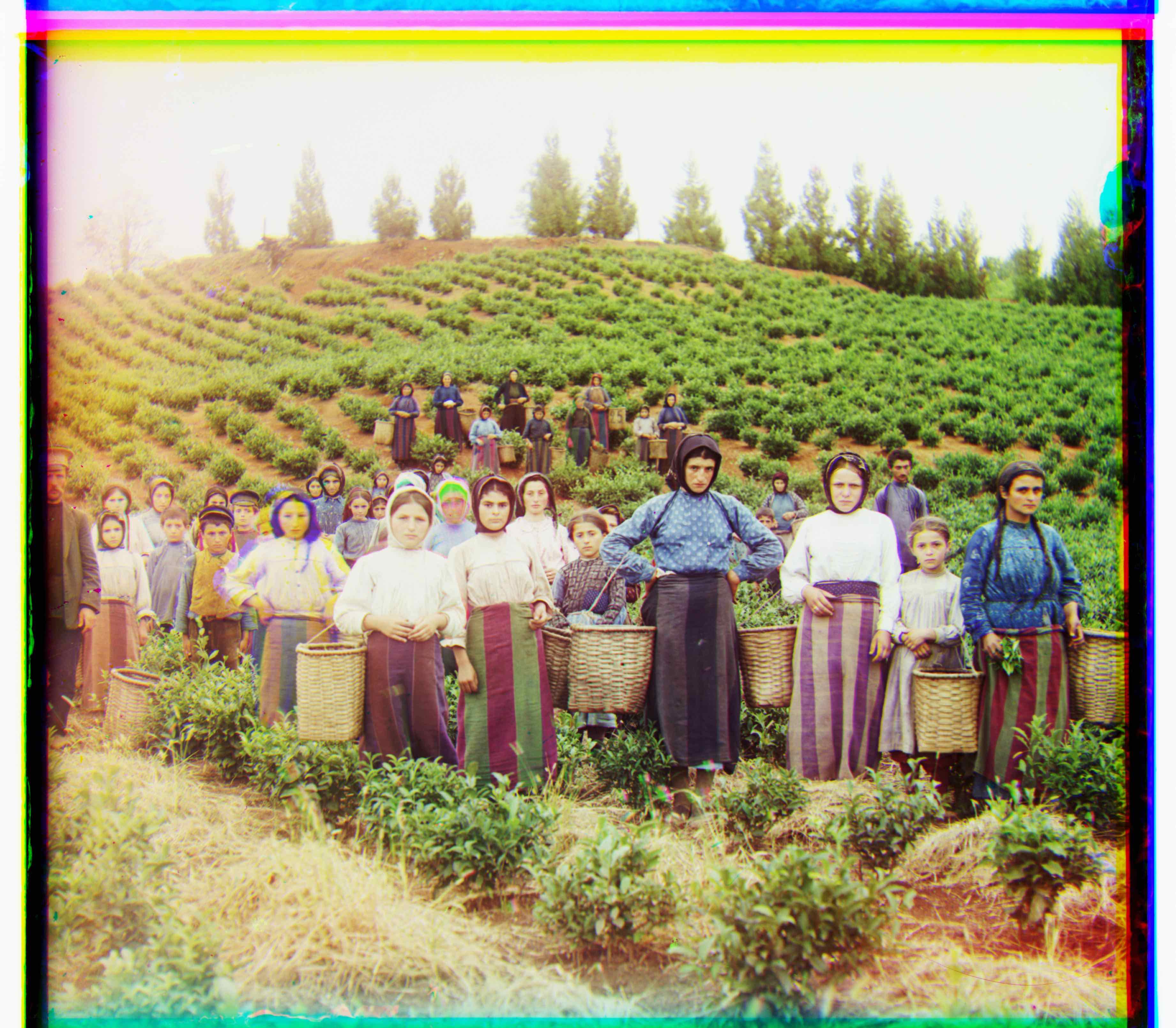
harvesters.tif
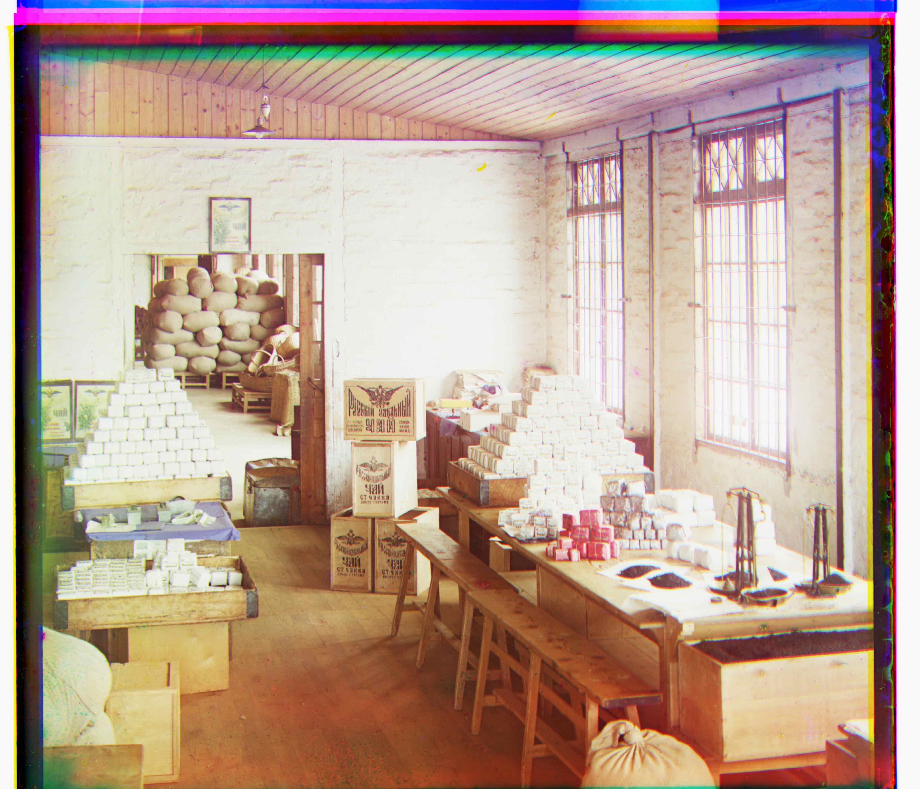
workshop.tif
g: (49, 24); r: (104, 5)
g: (60, 16); r: (125, 14)
g: (53, -1); r: (102, -13)
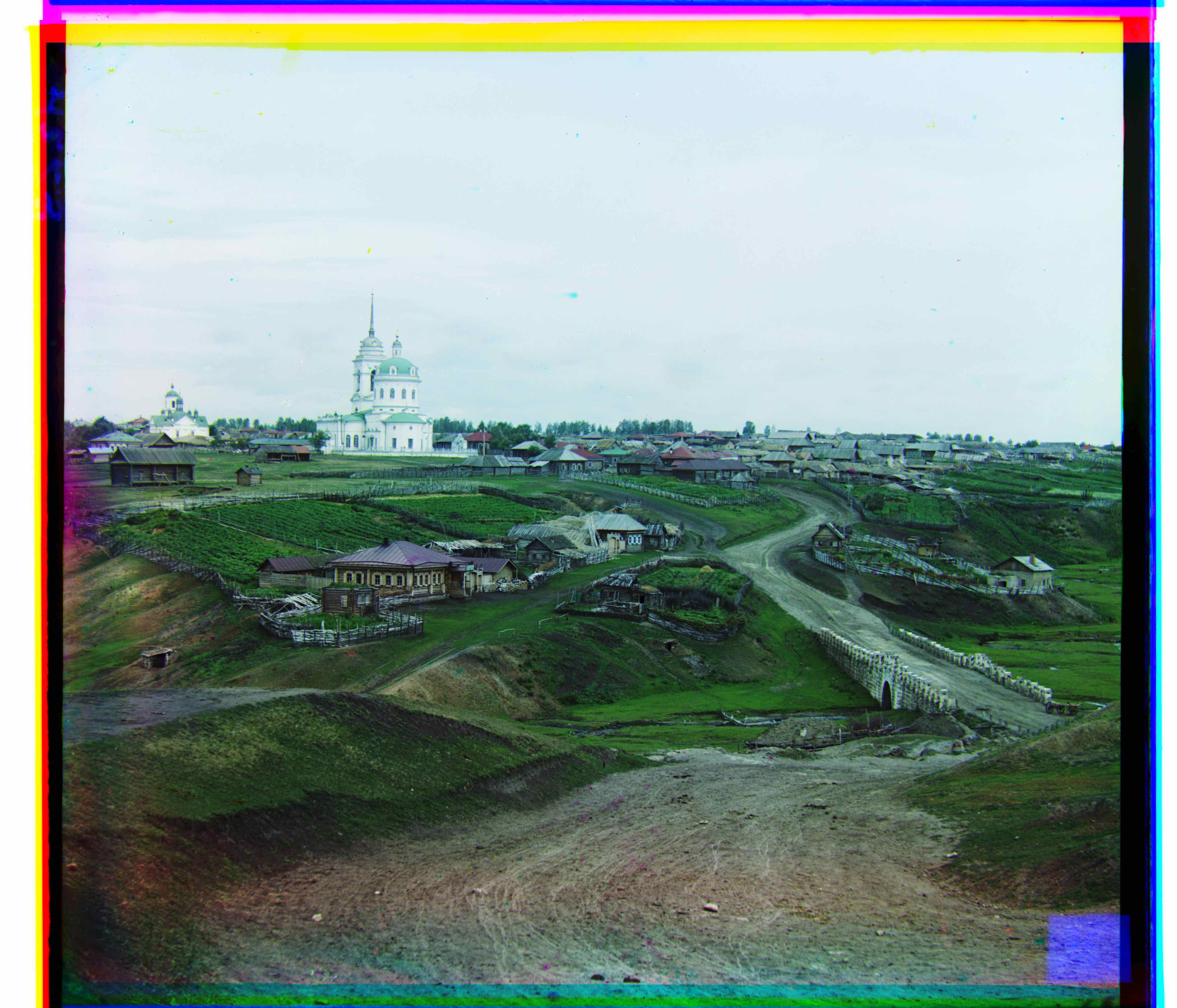
village.tif
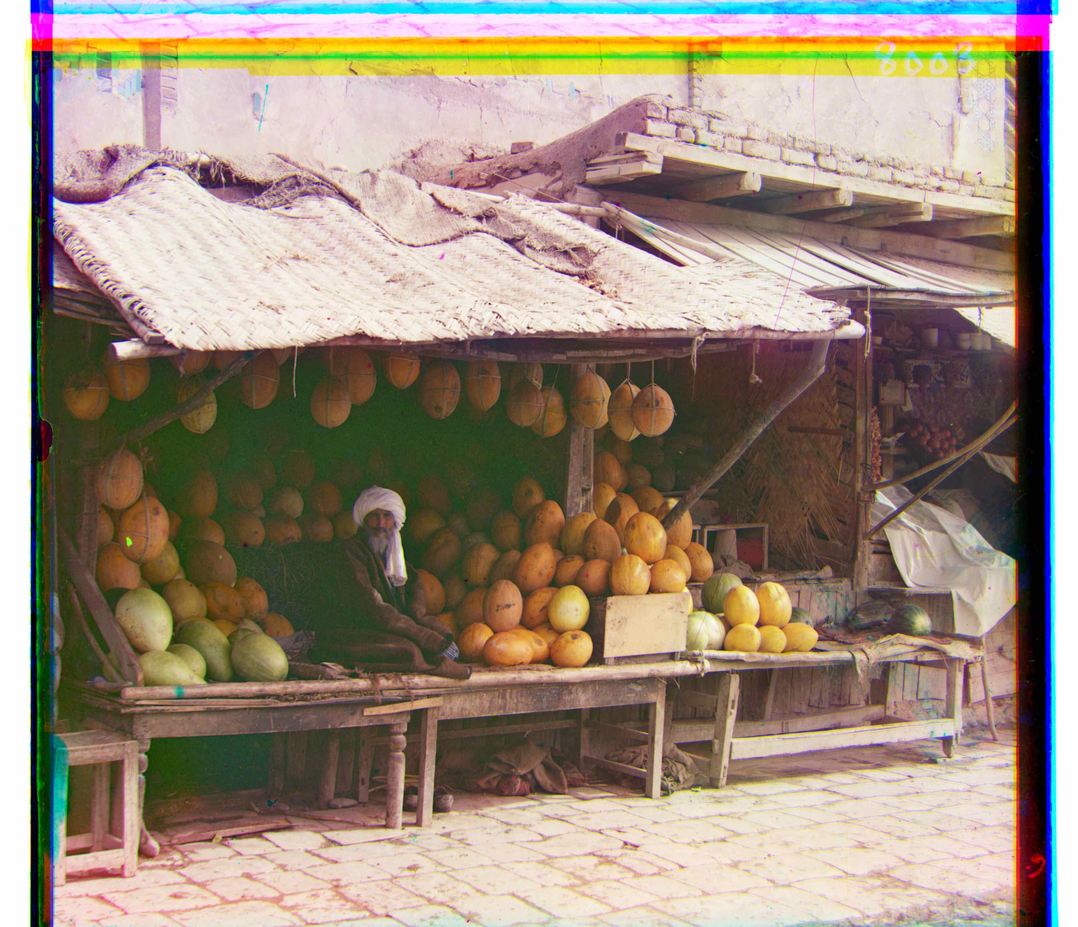
melons.tif
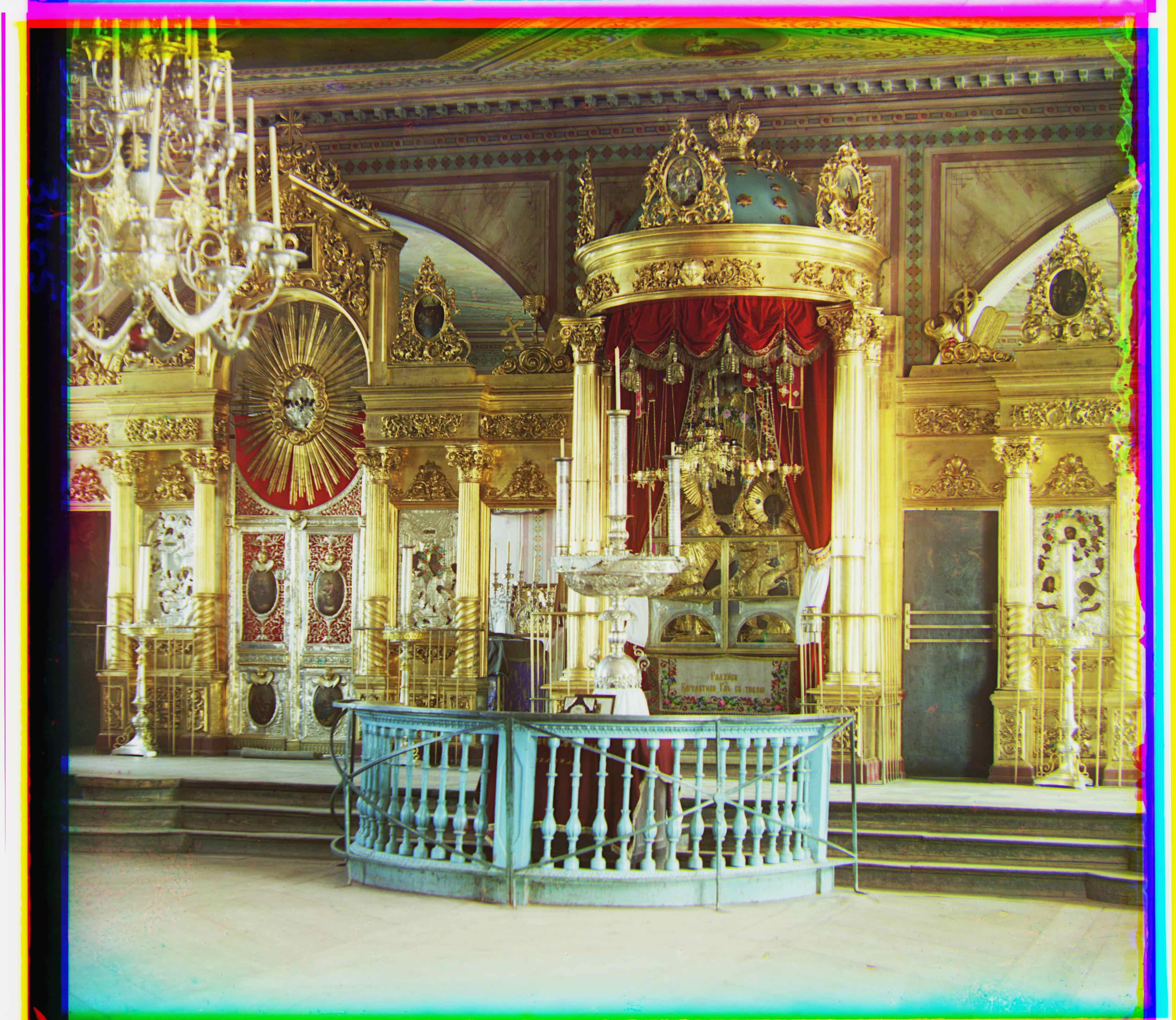
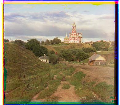
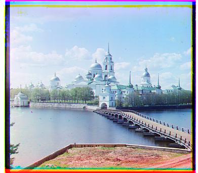
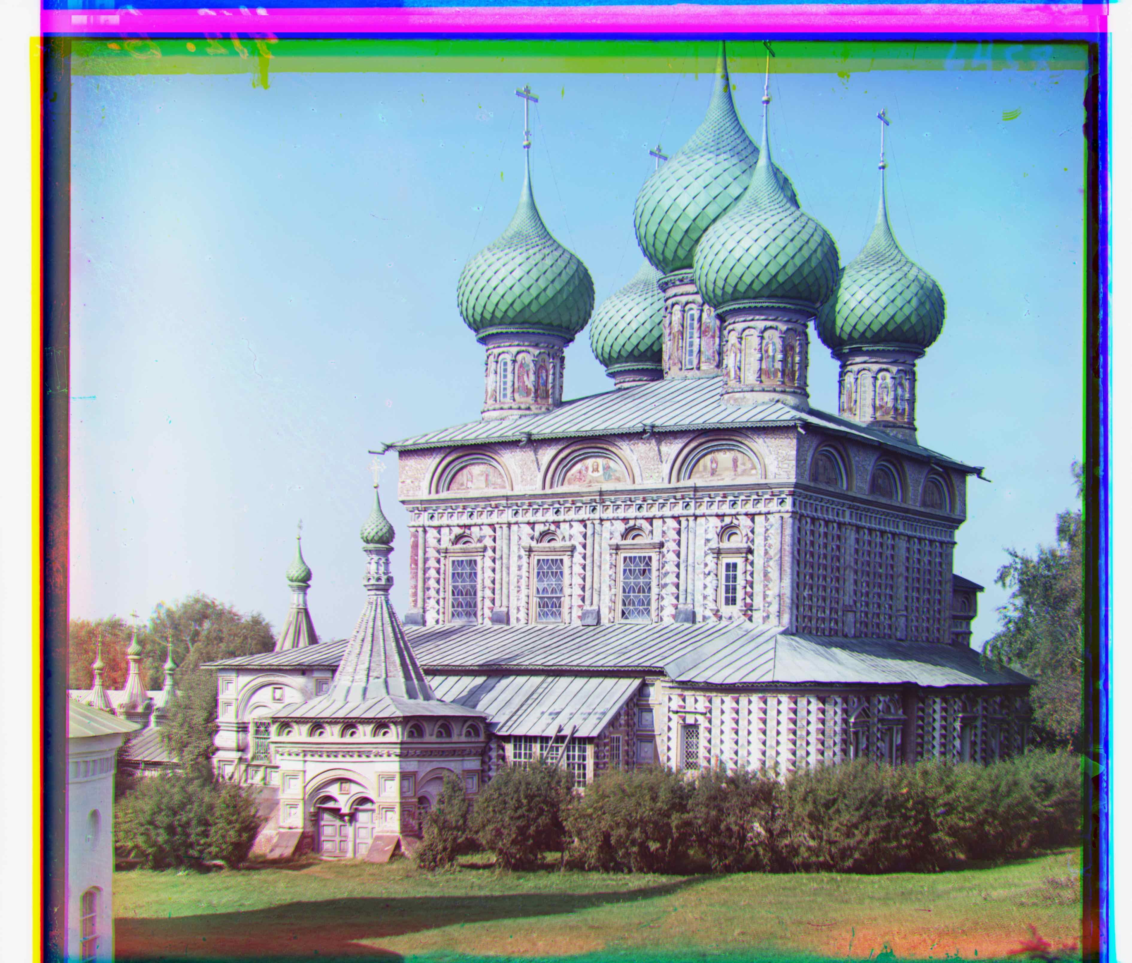
onion_church.tif
g: (65, 12); r: (138, 23)
g: (82, 8); r: (178, 11)
g: (51, 26); r: (108, 36)
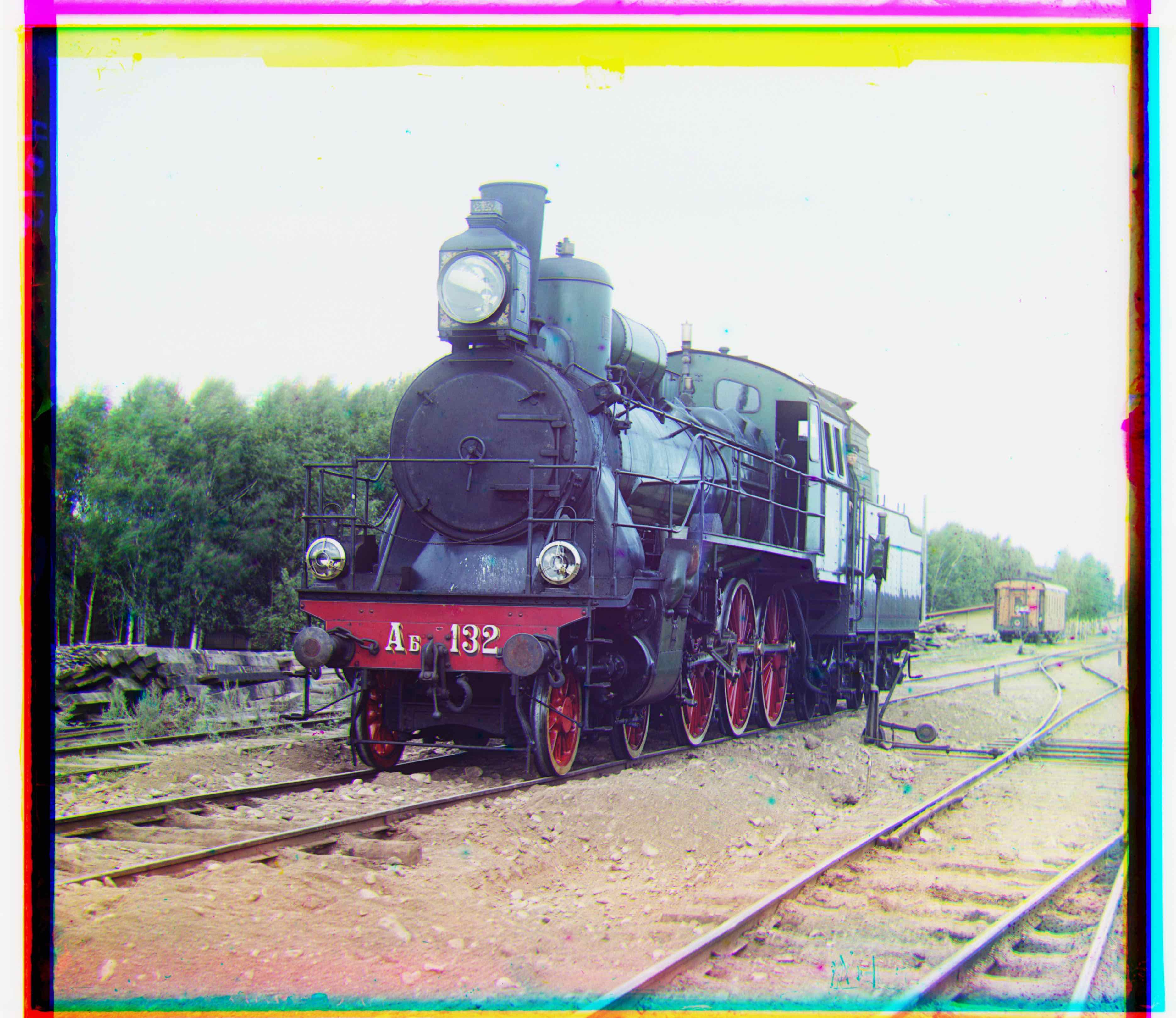
train.tif
three_generations.tif
g: (43, 6); r: (87, 32)
g: (55, 12); r: (112, 10)

Extra Results
For some images, balancing between the contrasted and uncontrasted versions seems to create more realistic results. Some examples are showed below.

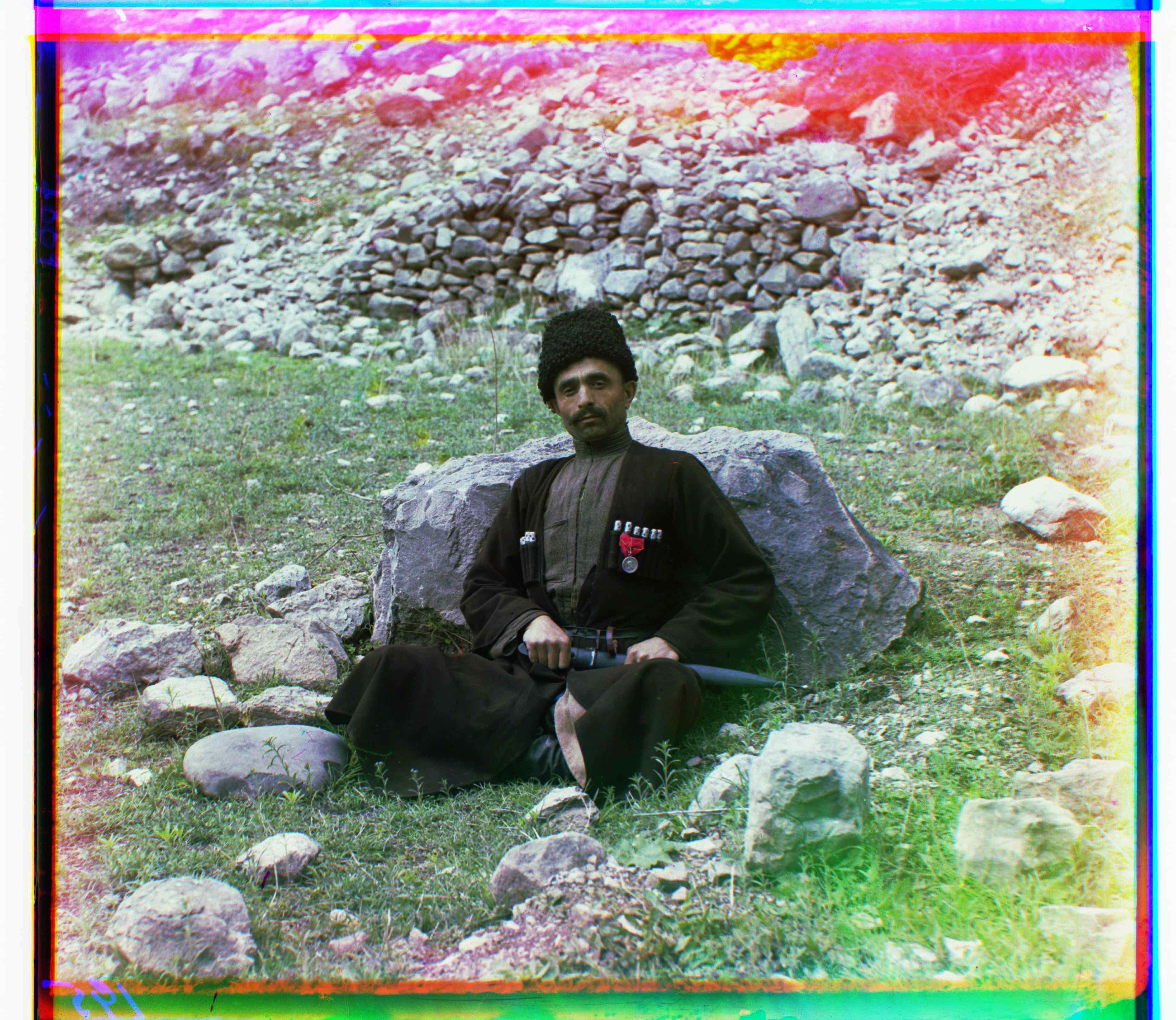
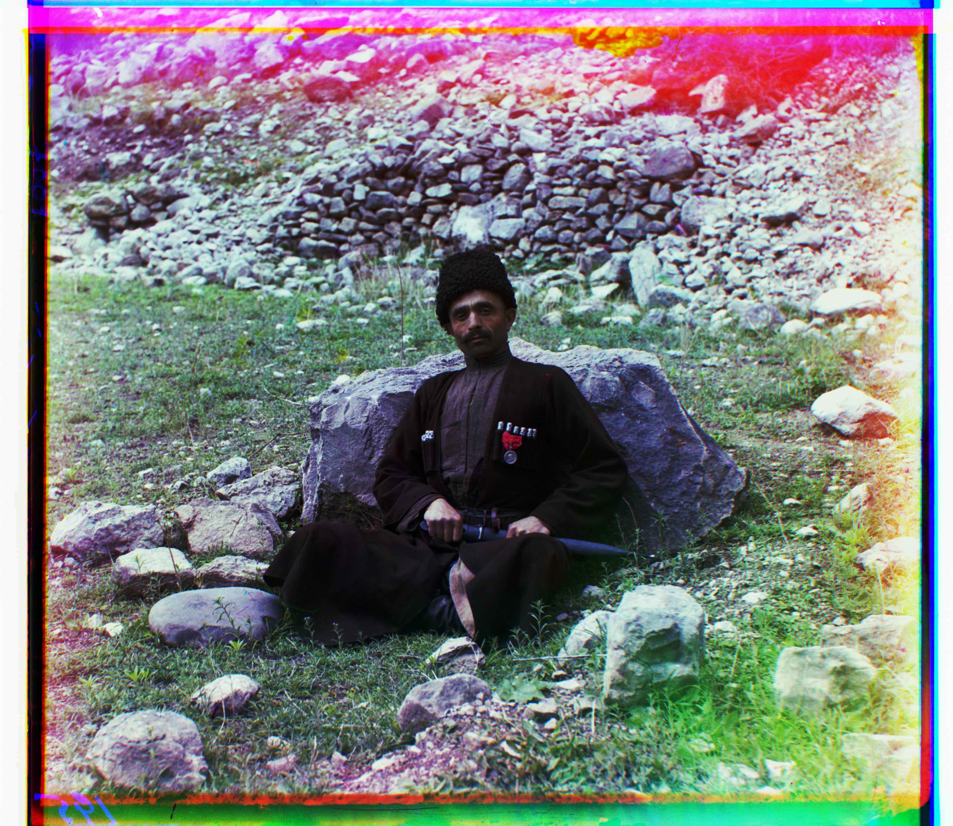

image1: without contrasting
image2: with contrasting
0.3 * image1 + 0.7 * image2