Proj 1 Images of the Russian Empire
Cheng (Bob) Cao
Overview
This project is a program that takes three monochrome films captured using colored filters and align & combine them into a resulting image.
Algorithm
The Basic Algorithm
def similaity_index(x, y)
    ...
end

def align (imageA, imageB)
    max_similarity = imageA
    dx = 0
    dy = 0

    for x in [-range .. range]
        for y in [-range .. range]
            similarity = similarity_index(offset(imageA, x, y), imageB)
            if similarity > max_similarity
                max_similarity = similarity
                dx = x
                dy = y
            end
        end
    end

    return dx, dy
end
The algorithm searches in a specified region of , offset the image A and compares it to image B. If the similarity is higher than the maximum we have recorded, we record the current offset and similarity as the maximum. After the search we return the offset.
The similarity function here can be any function that computes similarity between two images, ideally image B will be the target and the function calculates spatial similarity in order to align the image properlly. Here we use Sum Squared Distance (SSD) as the metric, and we align the Red and Blue image to the Green image as a target.
The Green image is chosen as a target because it is the brightest perceived color in natural images and human vision. Green channel is often regarded as a brightness channel, which should give us a better target with lower noise.
Image Pyramid
Because the images could get very large, and for a offset, the image offset could be pixels in either direction. Searching over this radius could be extremely slow and painful. The solution here is image pyramid.
Image pyramid progressively downsample the images by a factor a and forms a "pyramid" of images. In graphics term this could be called MipMaps. We can perform search on the smallest image and progressively perform adjustments to the estimate when the image gets more granular. By using image pyramid, we can use a constant offset and even get much better performance on both large and small images.
In this implementation, a range of is used. As the image pyramid halfs the size of the images each time, this range would be sufficient as each level moves the image in same amount of offset as the previous image's pixel size. This is similar to how binar number representation works, we only need a very small adjustment per level to achieve a large and smooth range. As the search range per level is very small, this implementation is very fast and robust. Each image is processed under seconds.
Results
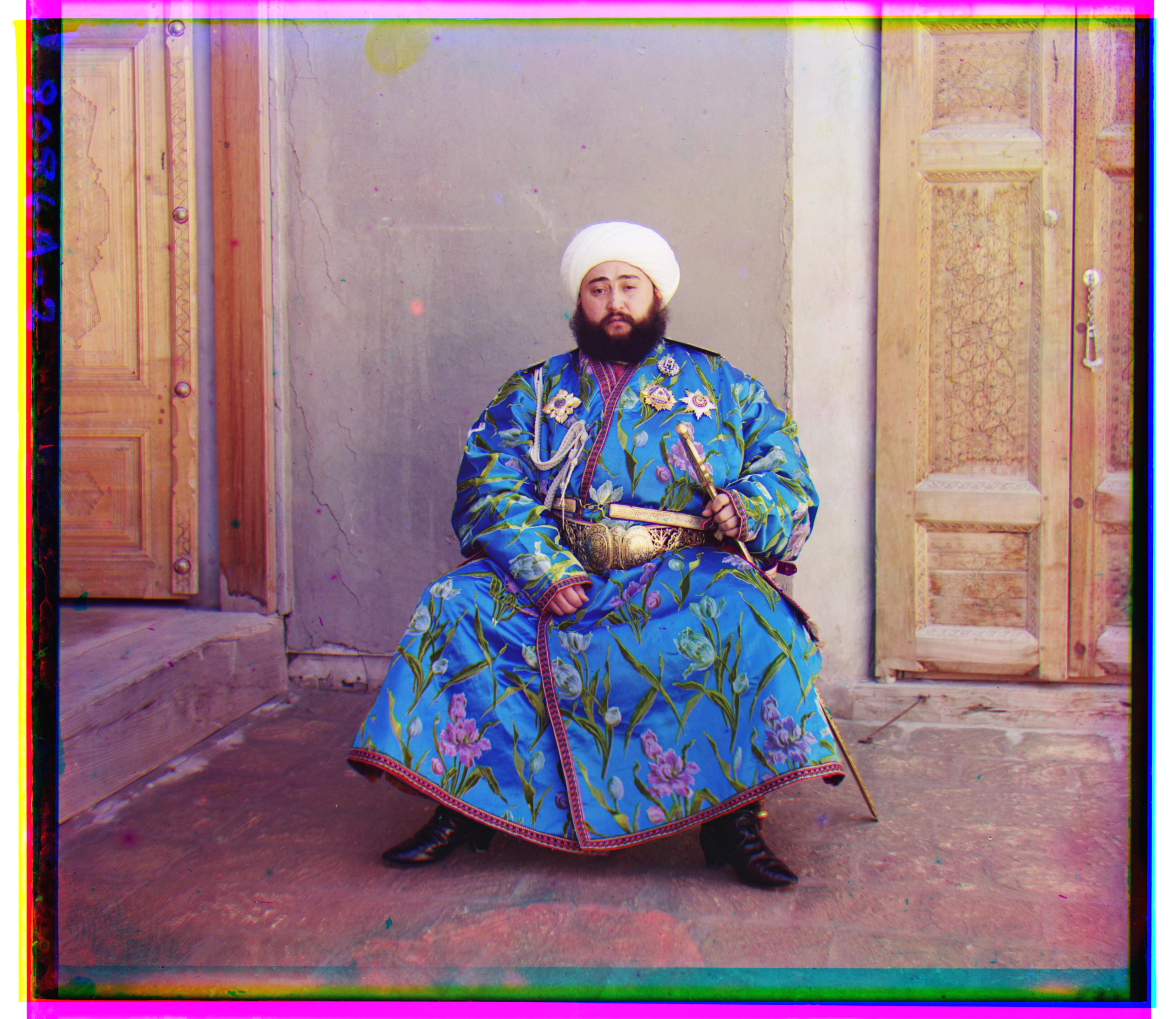
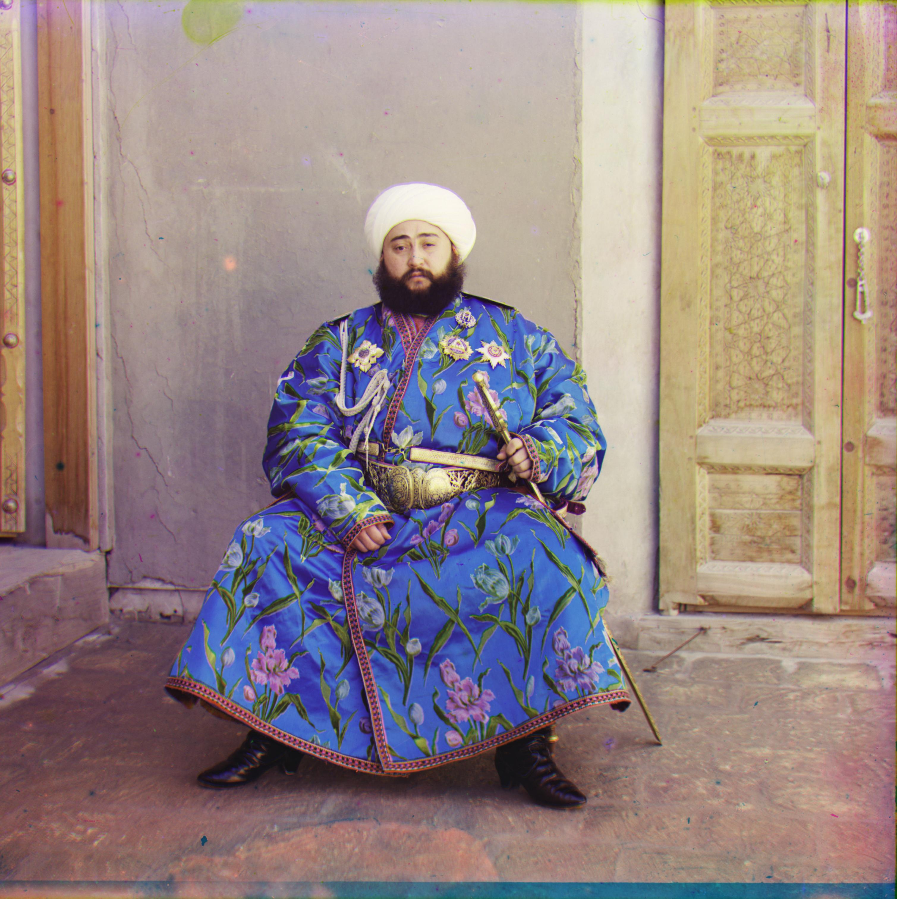
Emir: ,
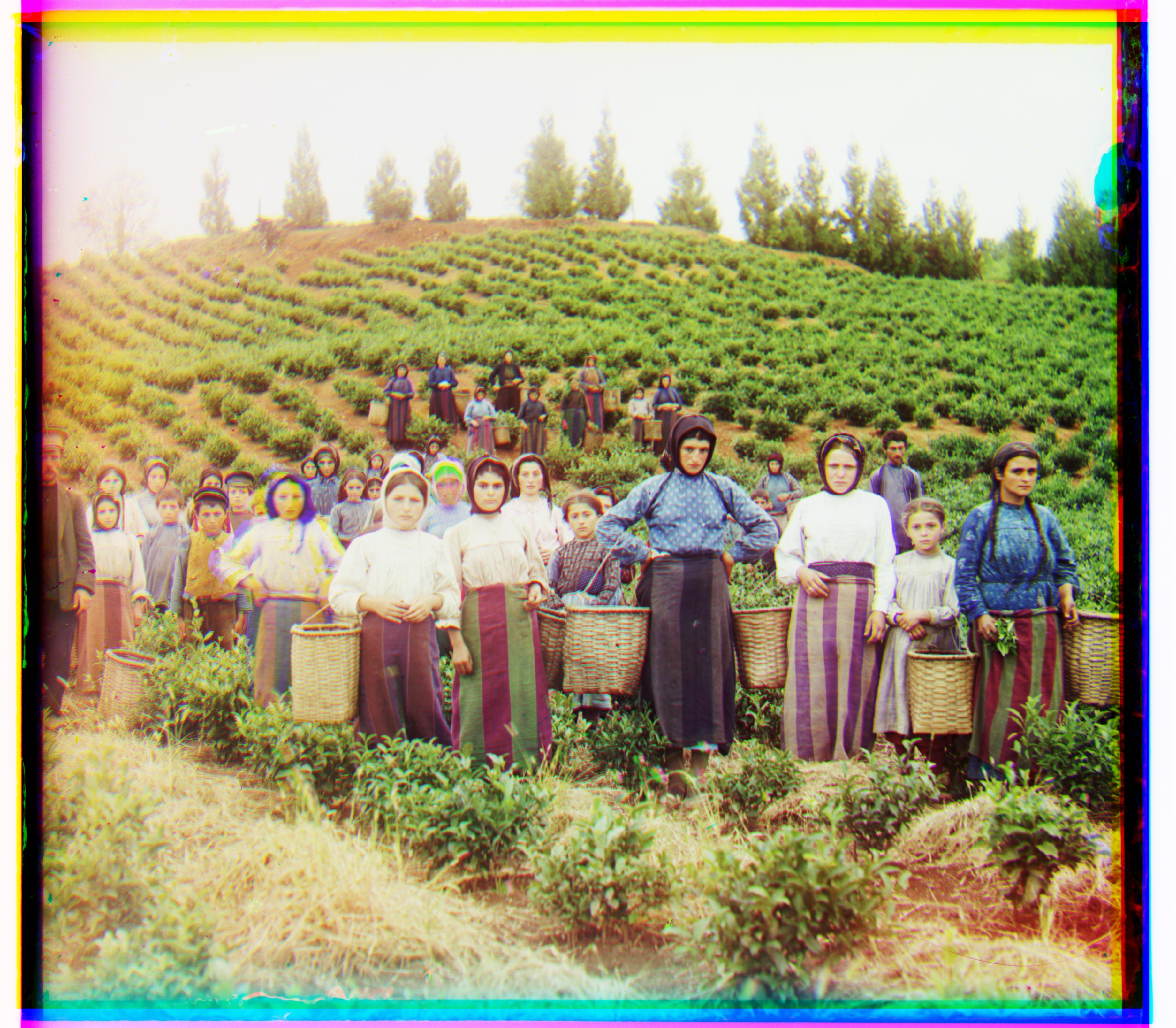
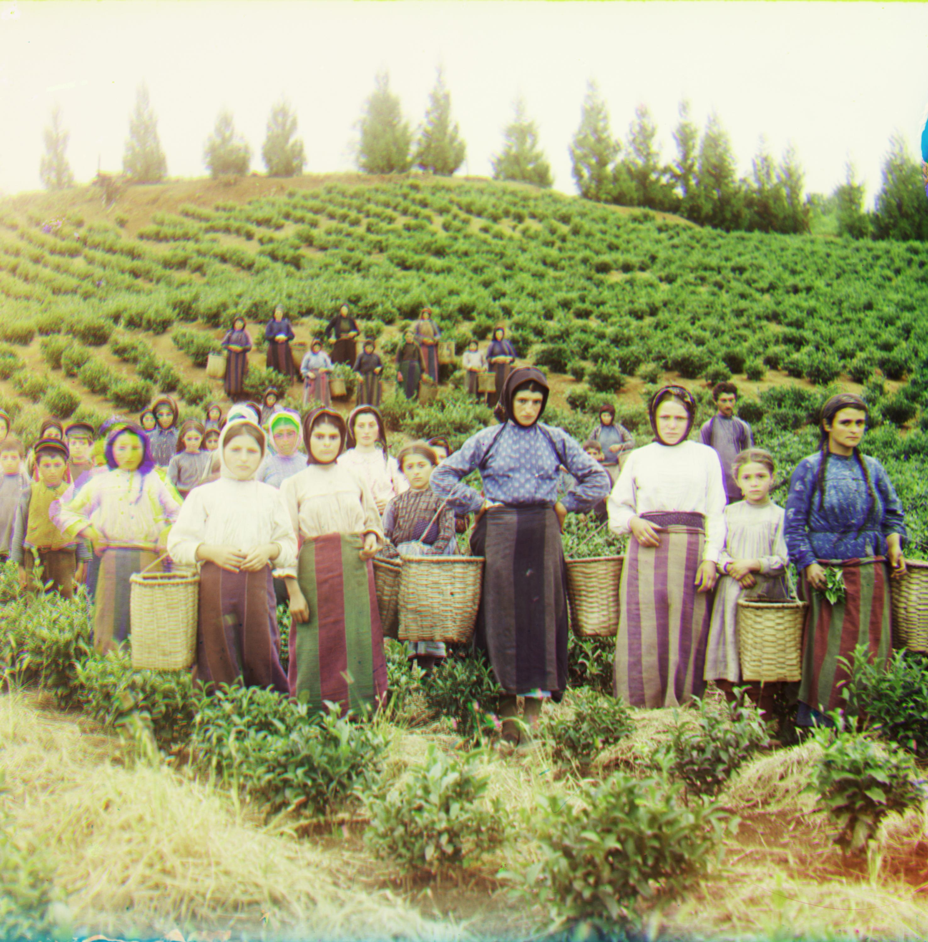
Harvesters: ,
Icon: ,
![]()
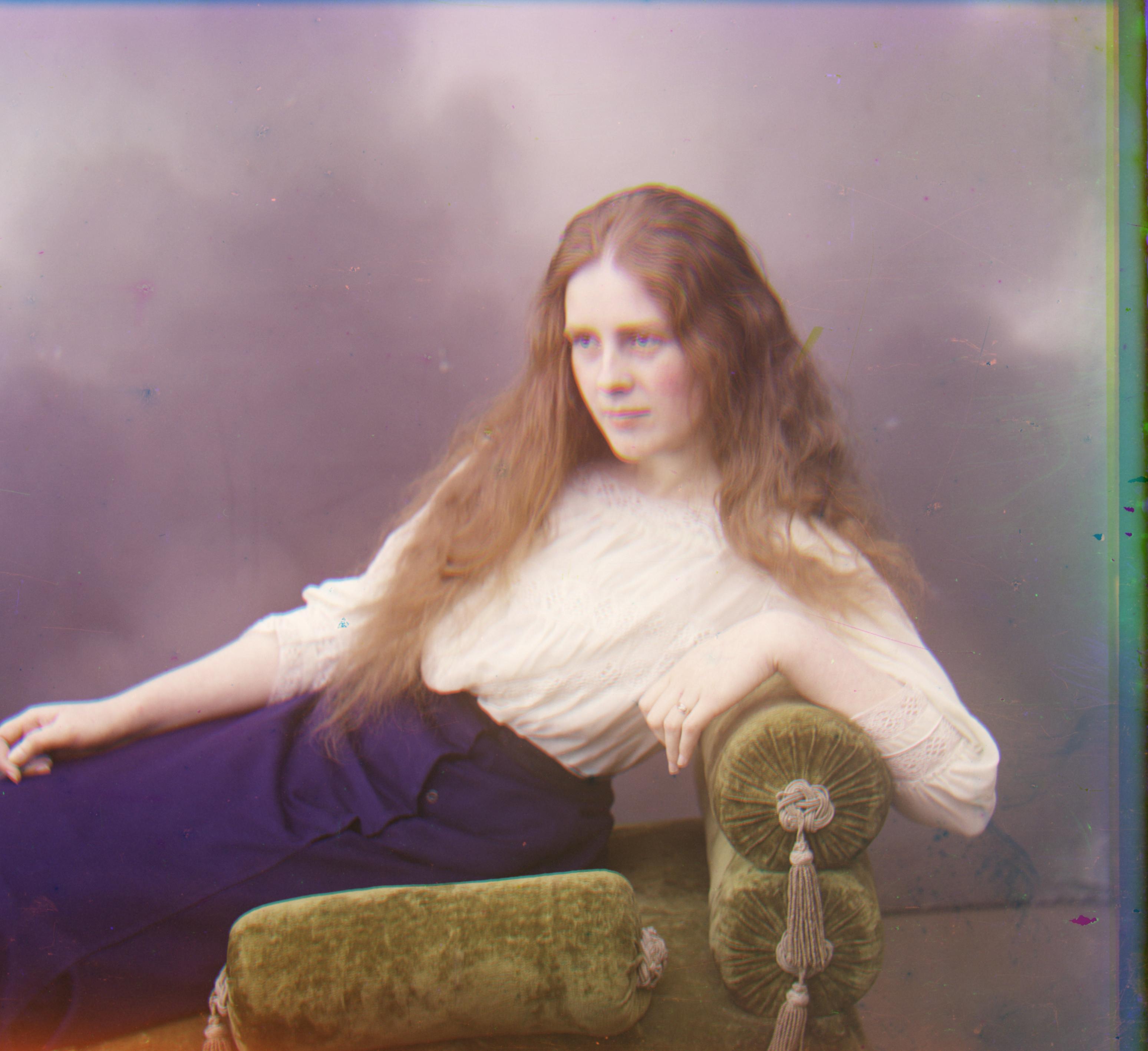
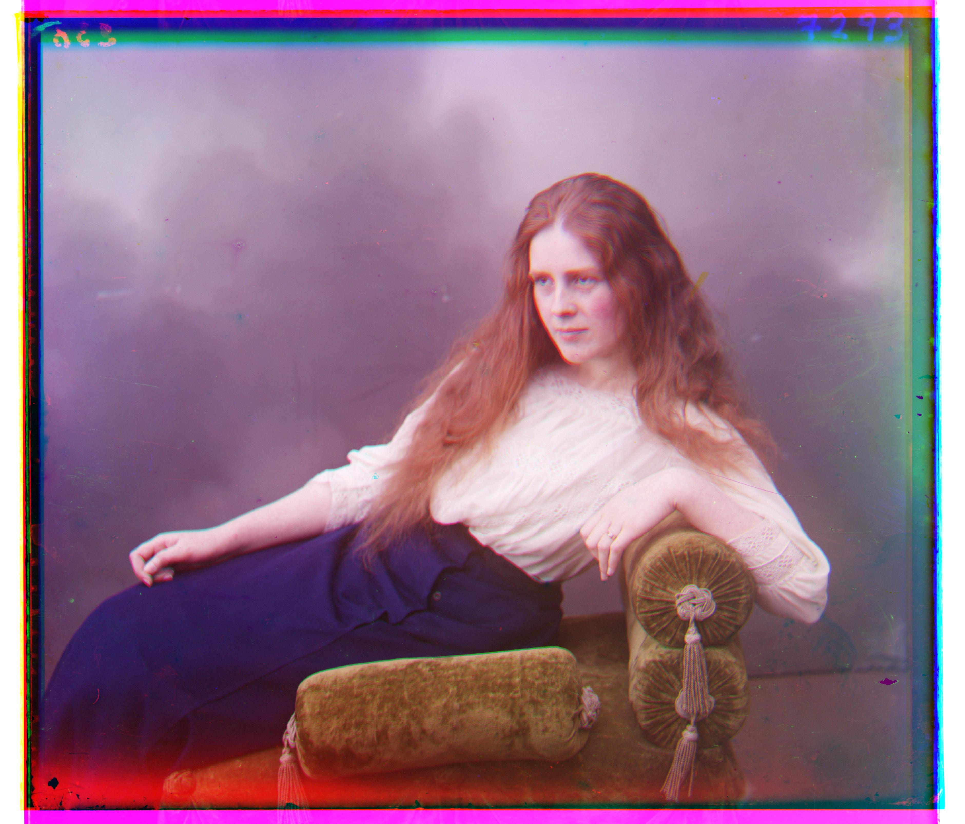
Lady: ,
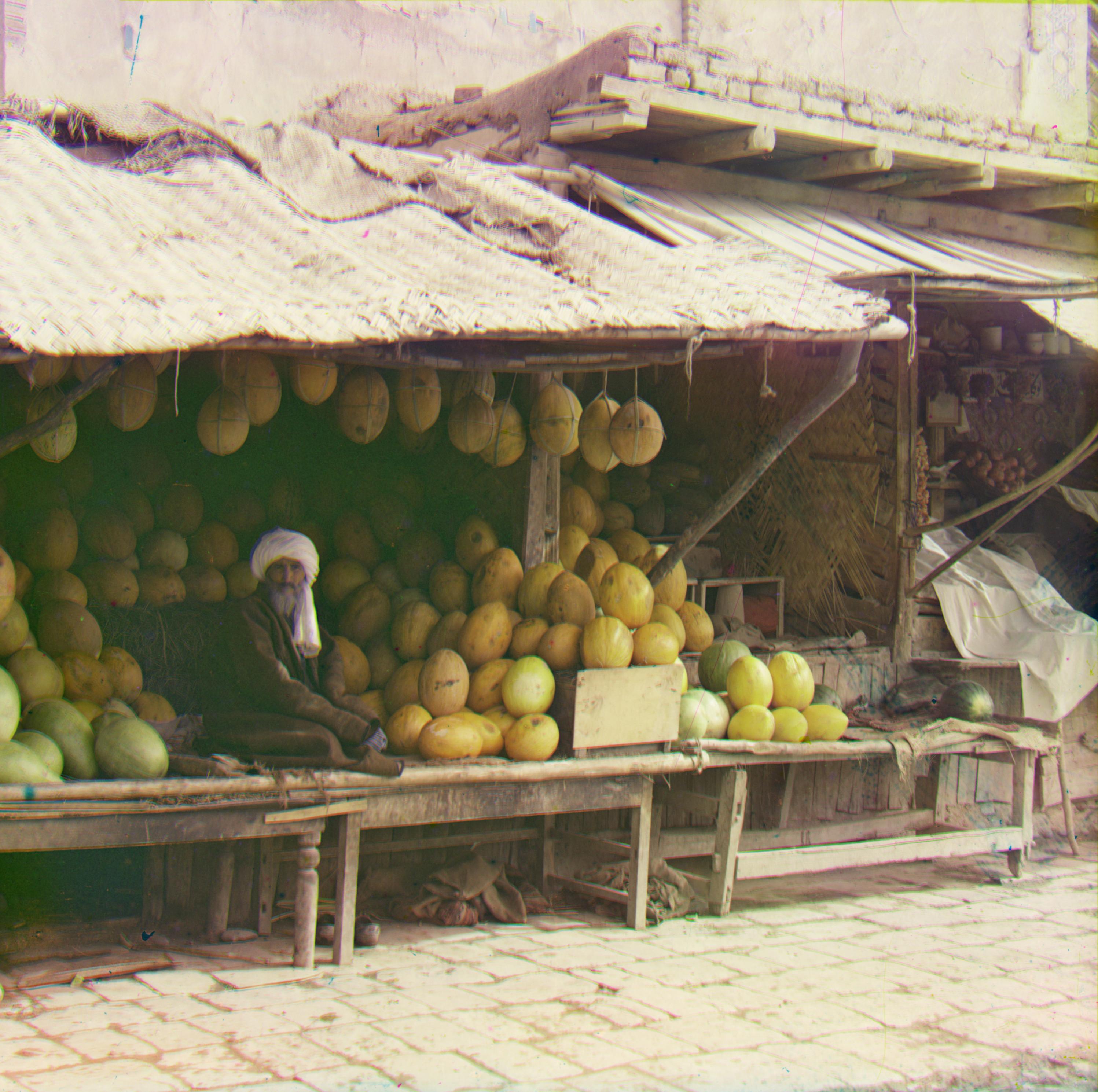
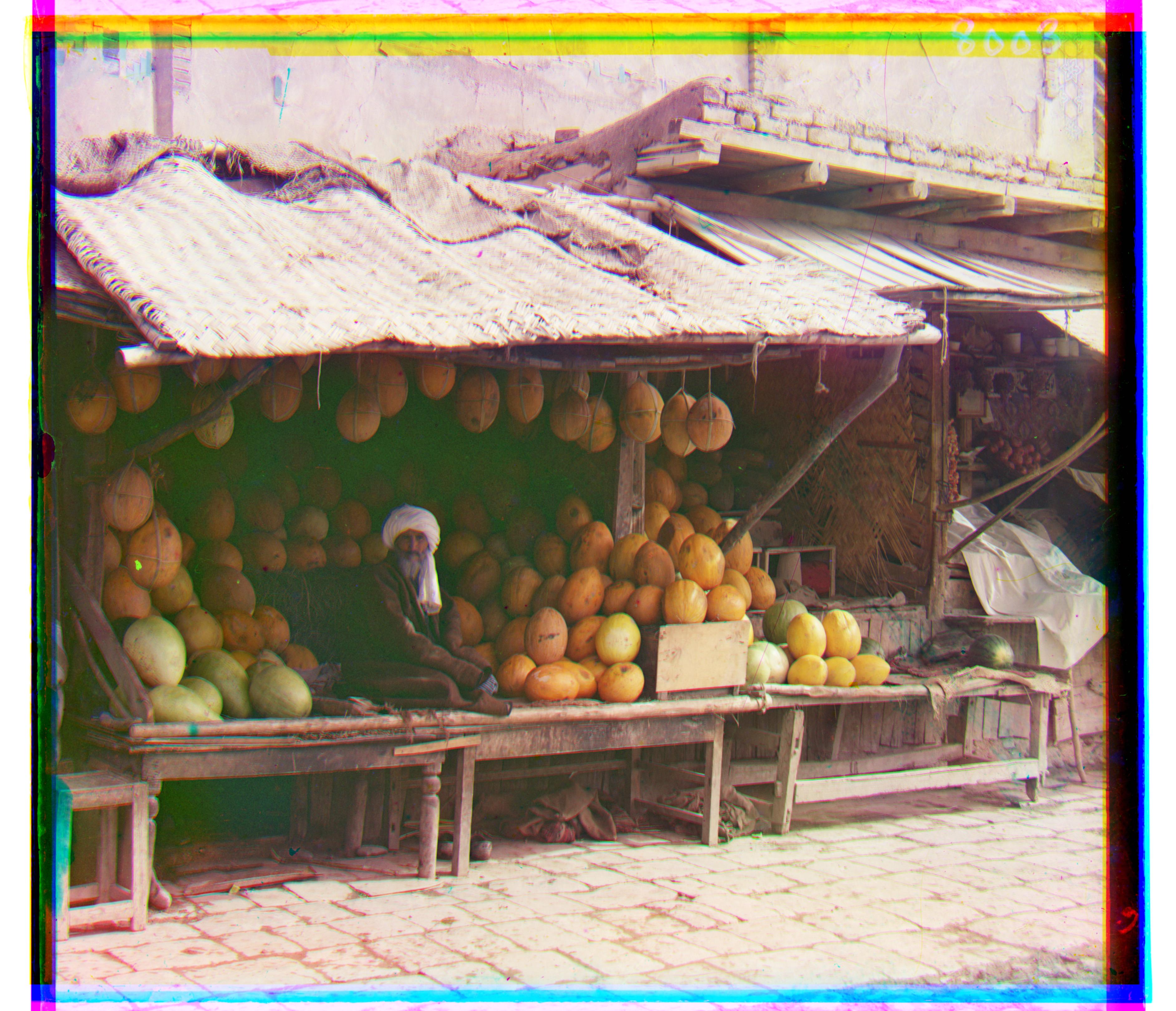
Melons: ,
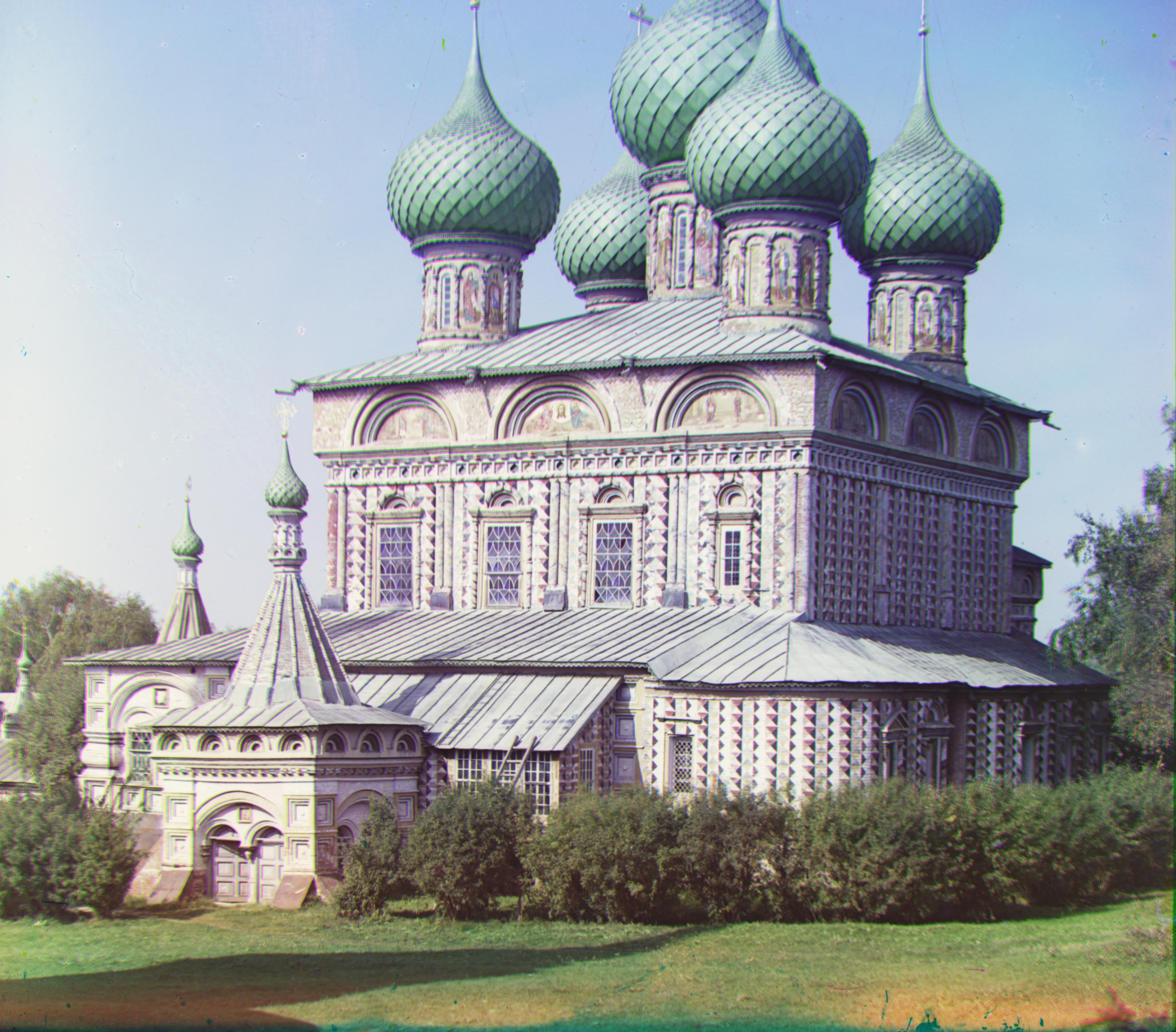
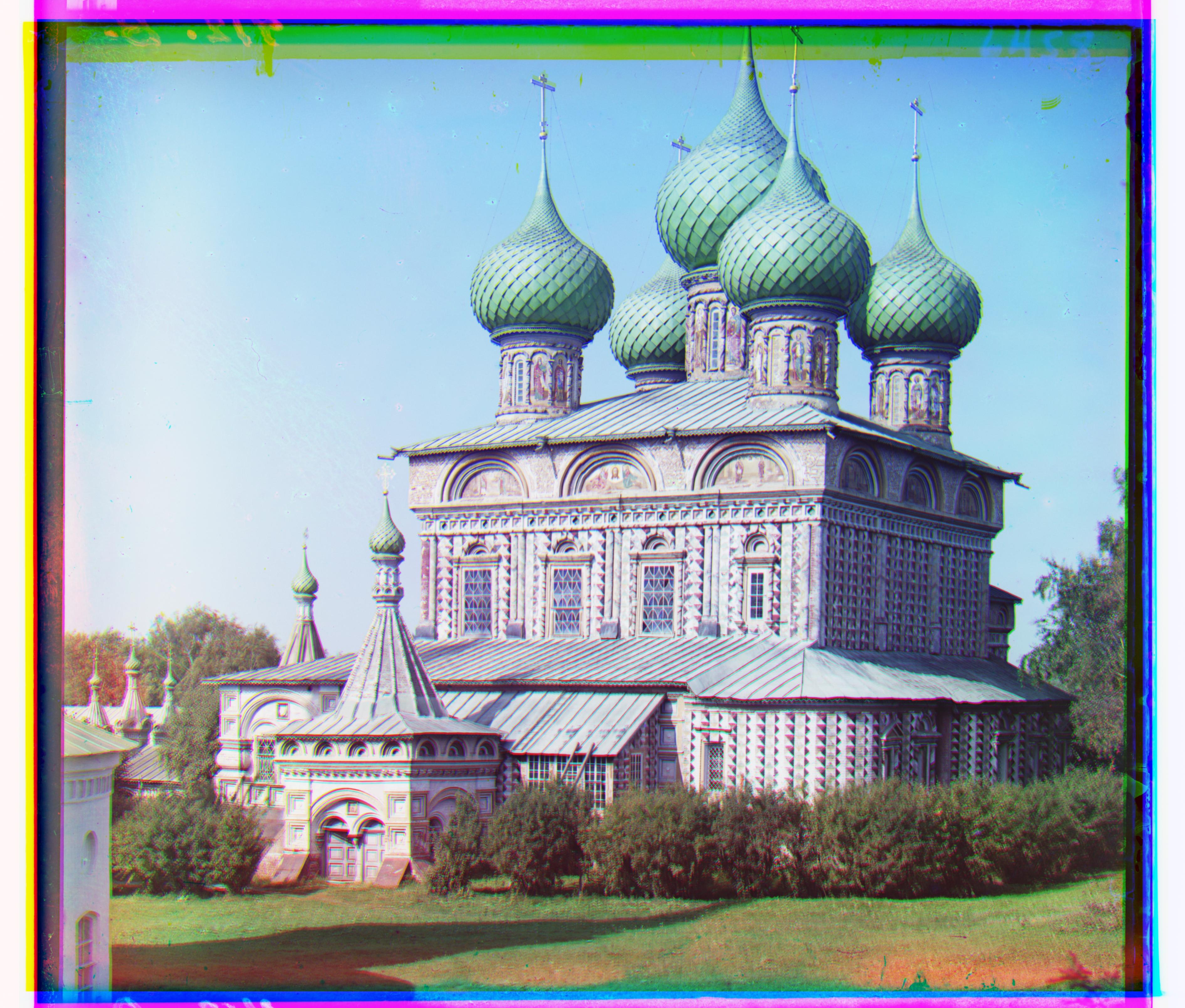
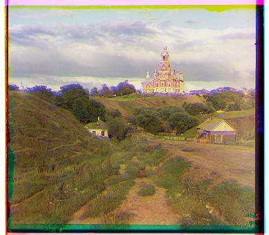
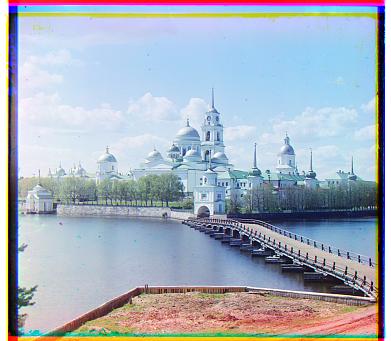
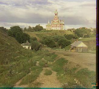
Onion Church: ,
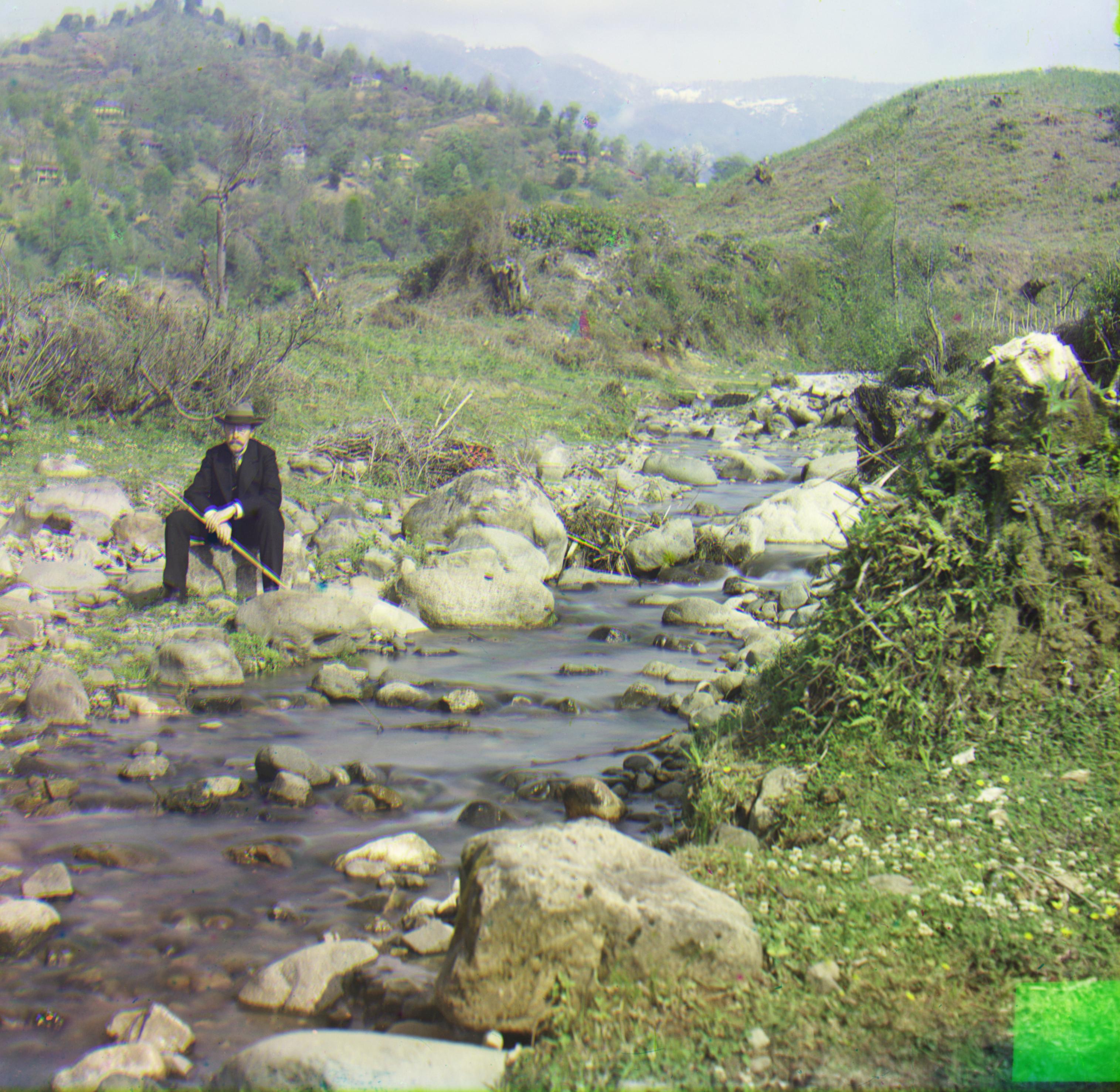
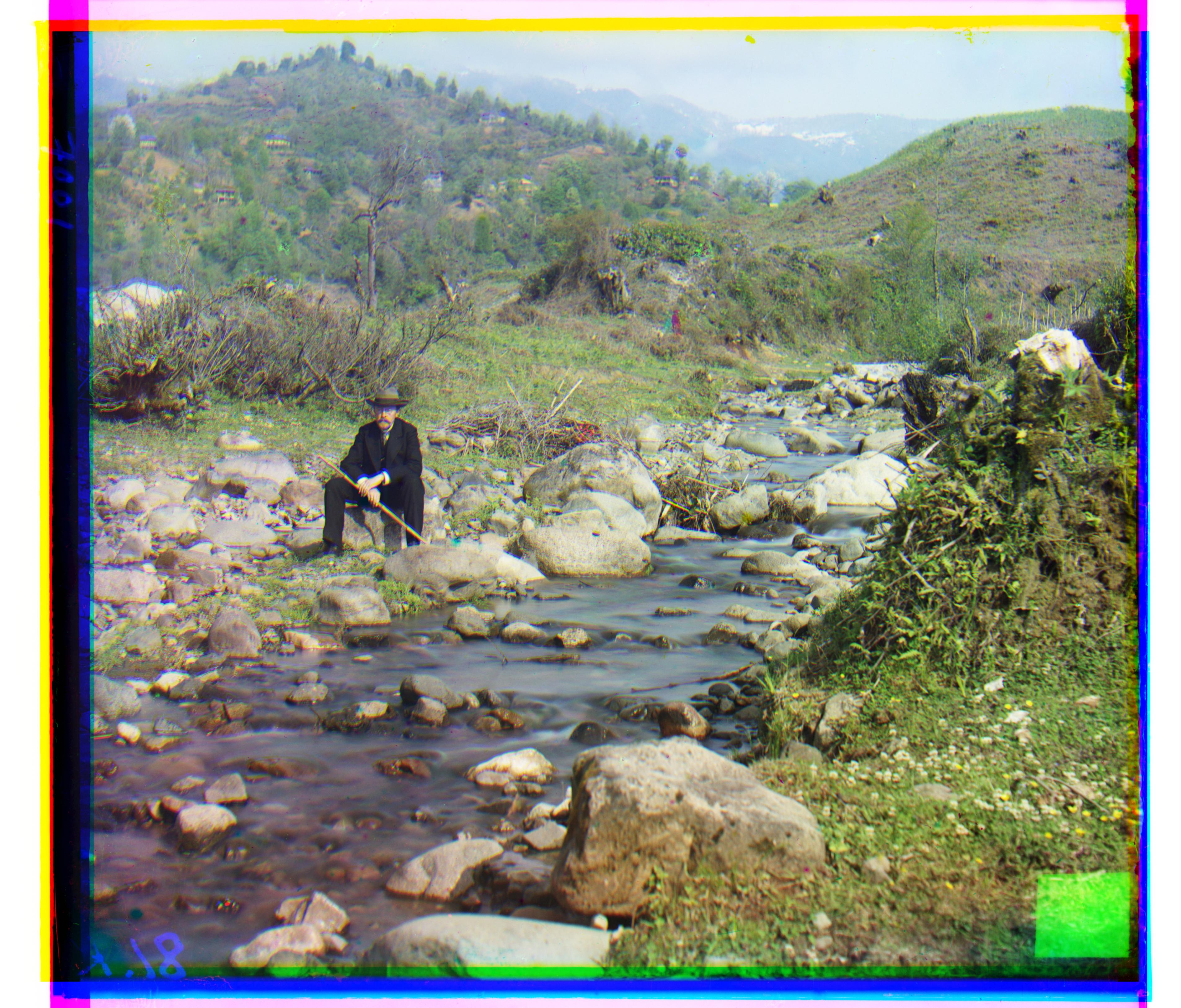
Self Portrait: ,
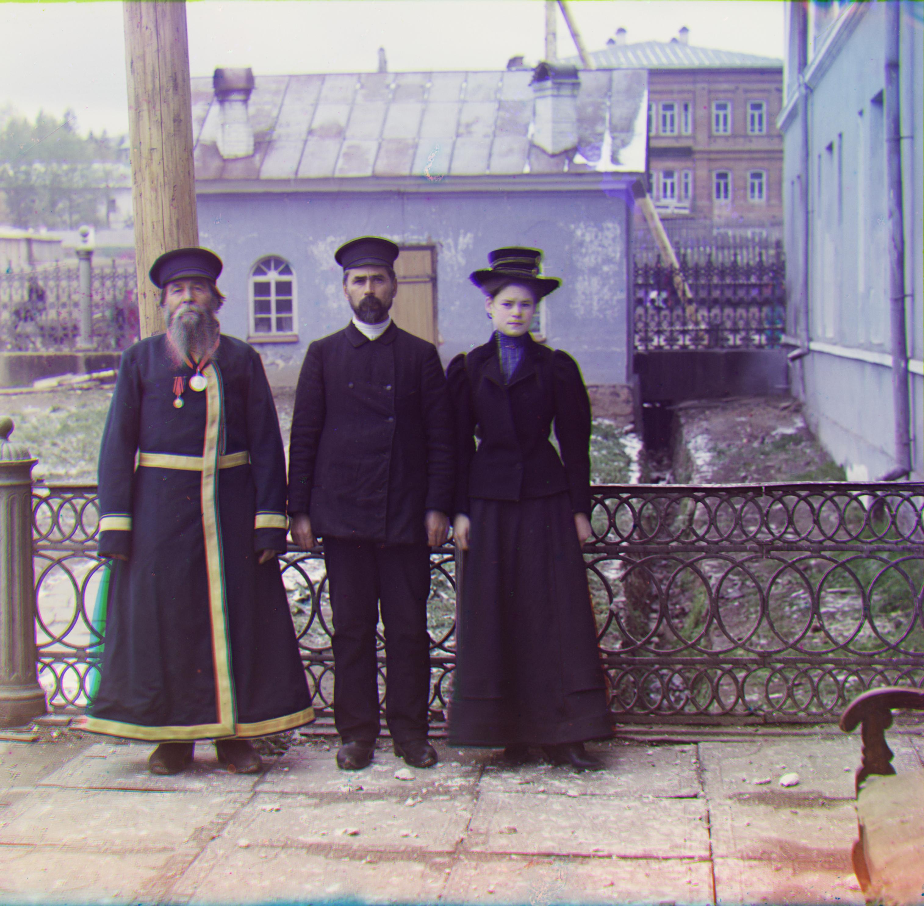
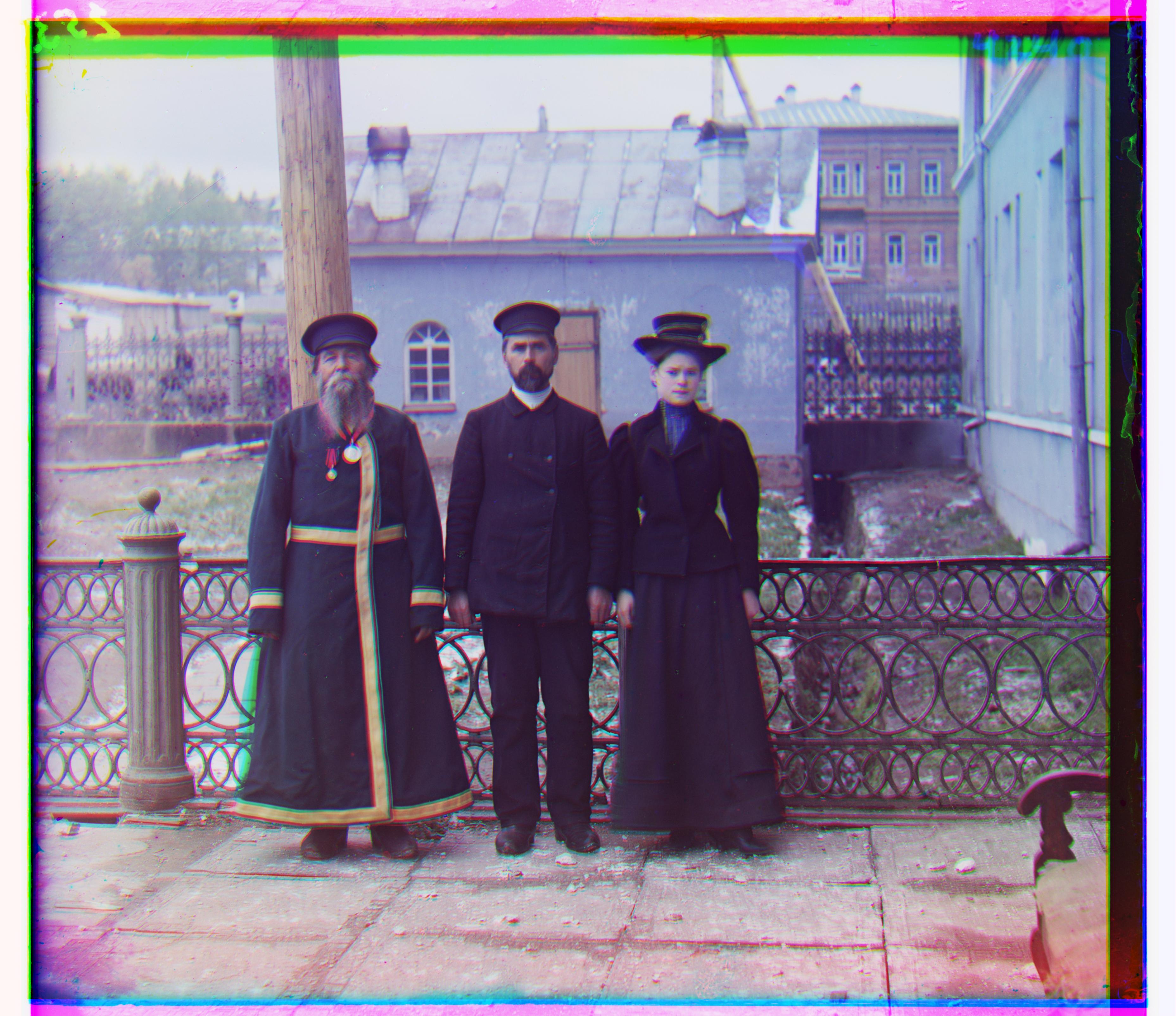
Three Generations: ,
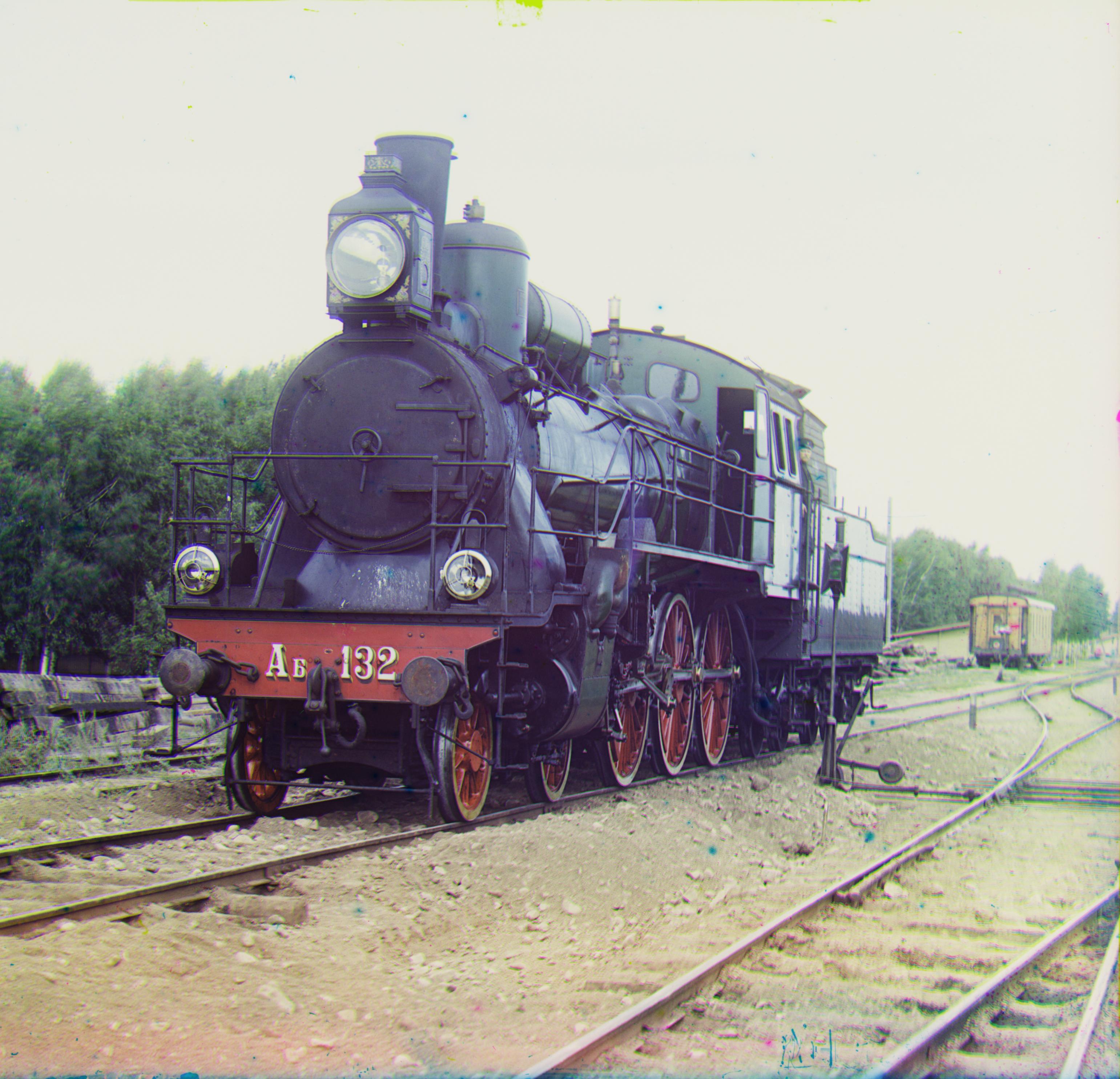
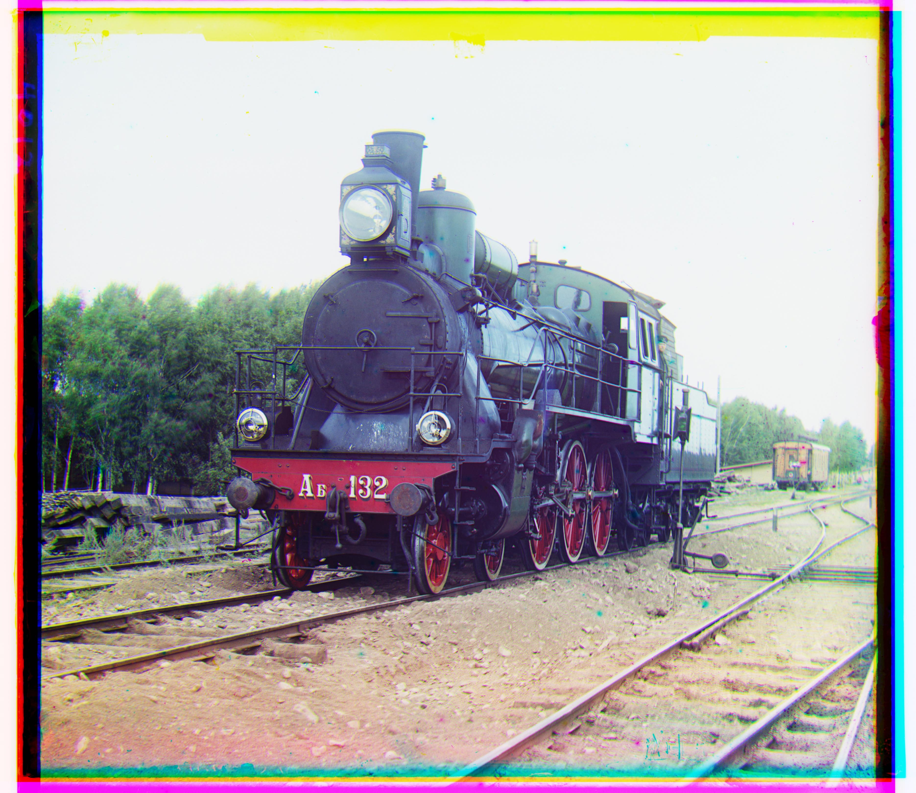
Train: ,
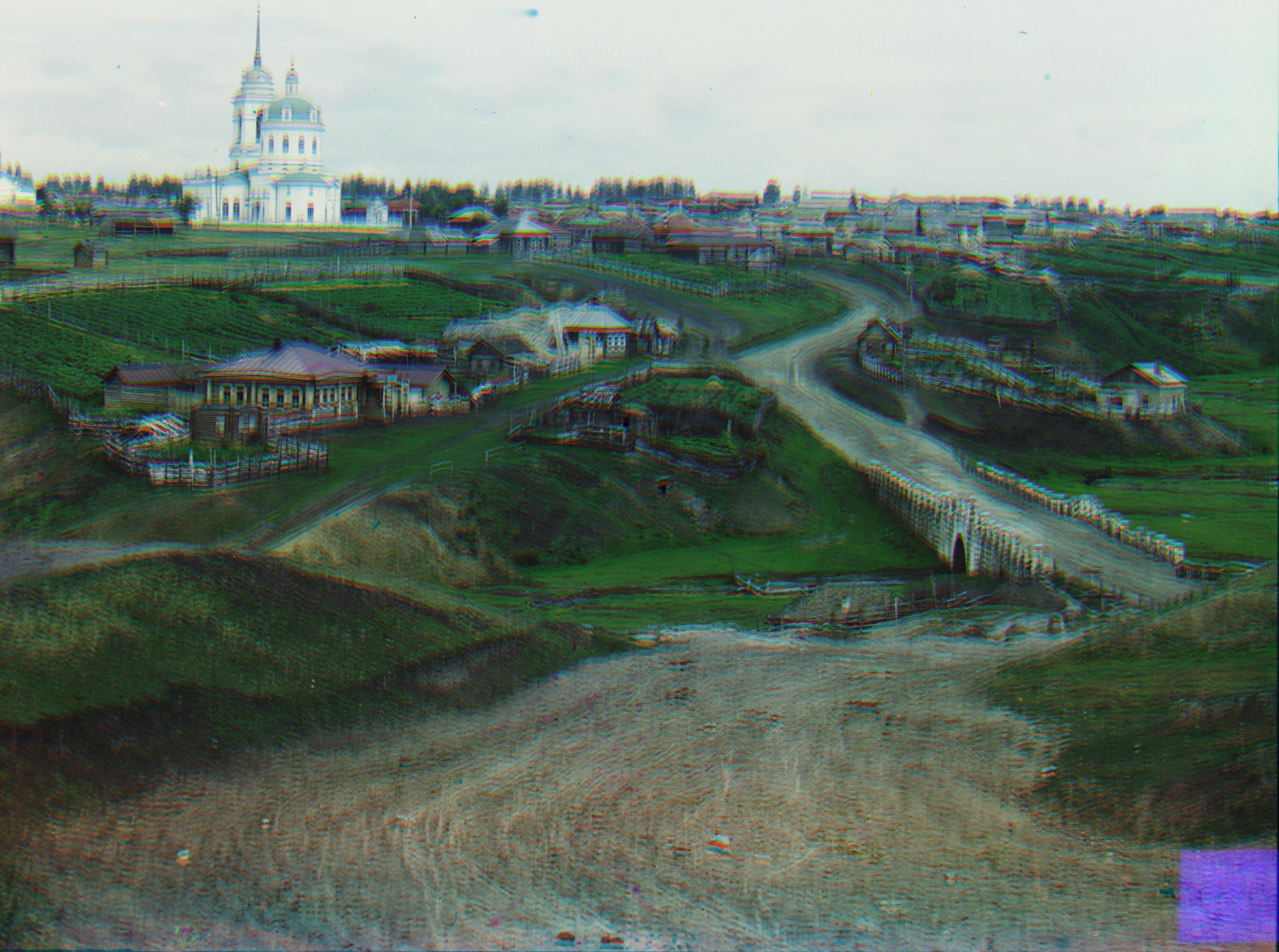
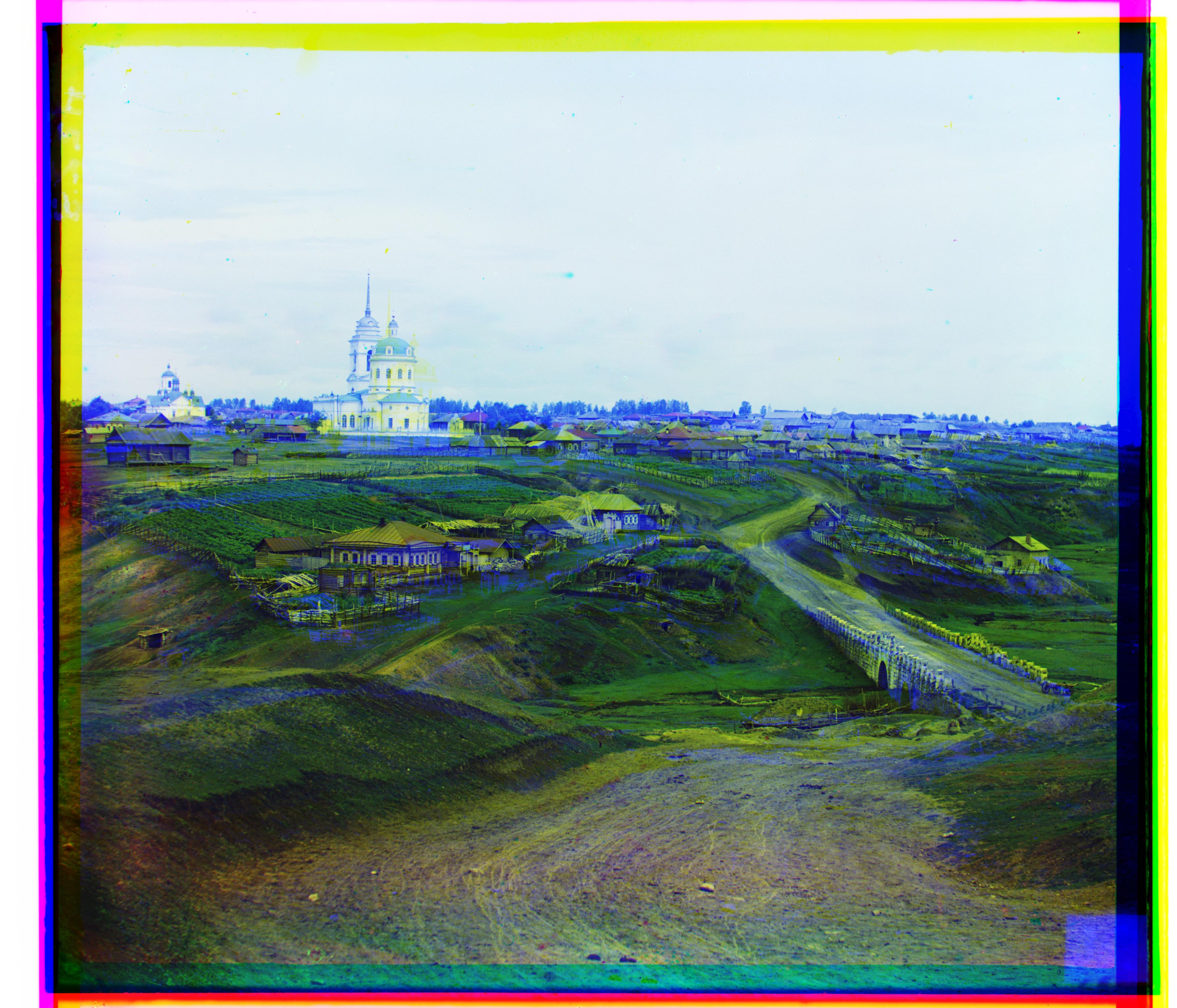
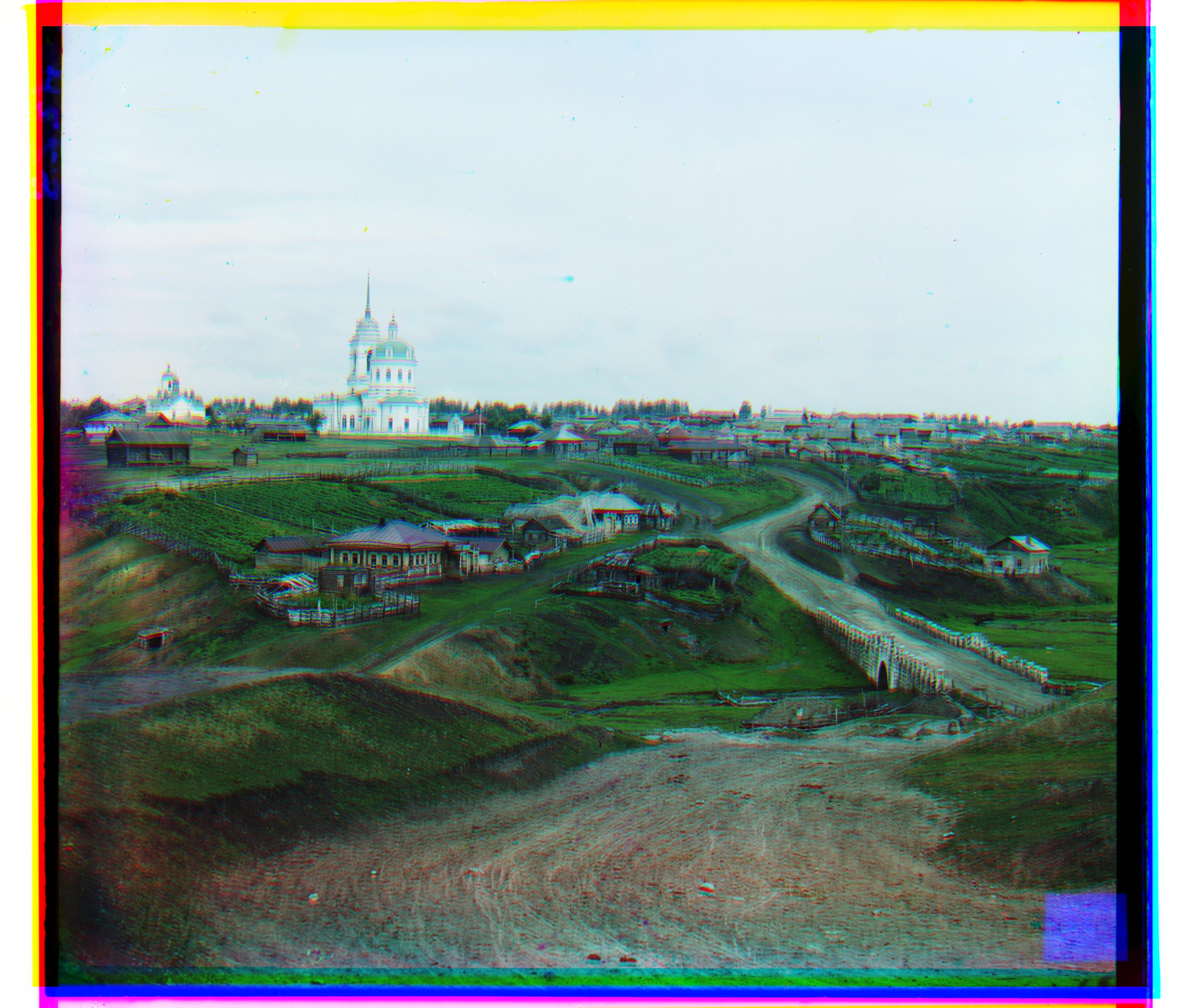
Village: ,
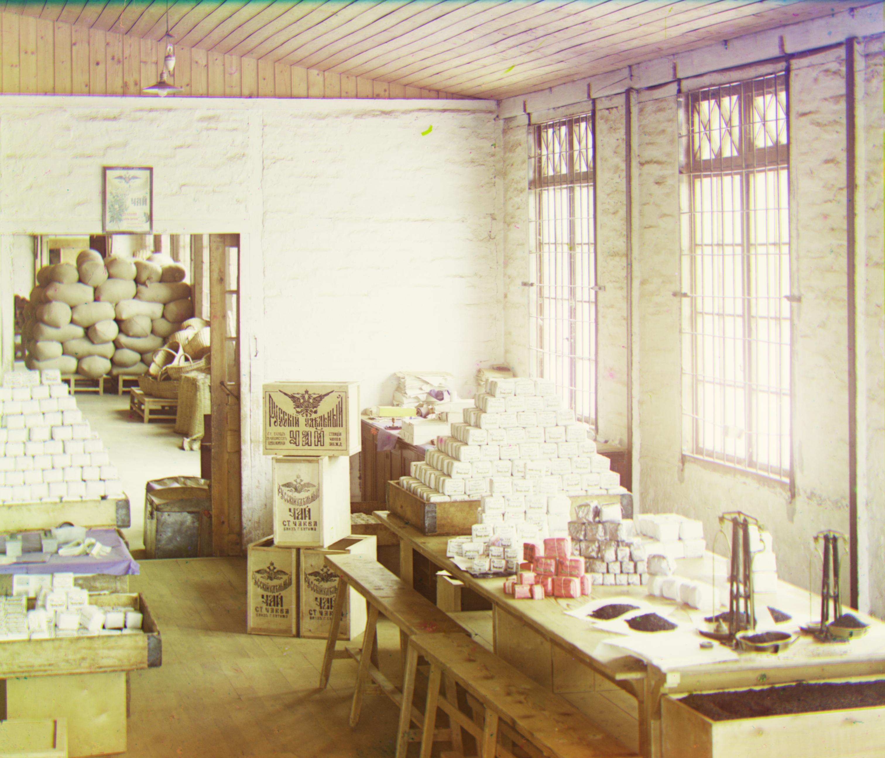
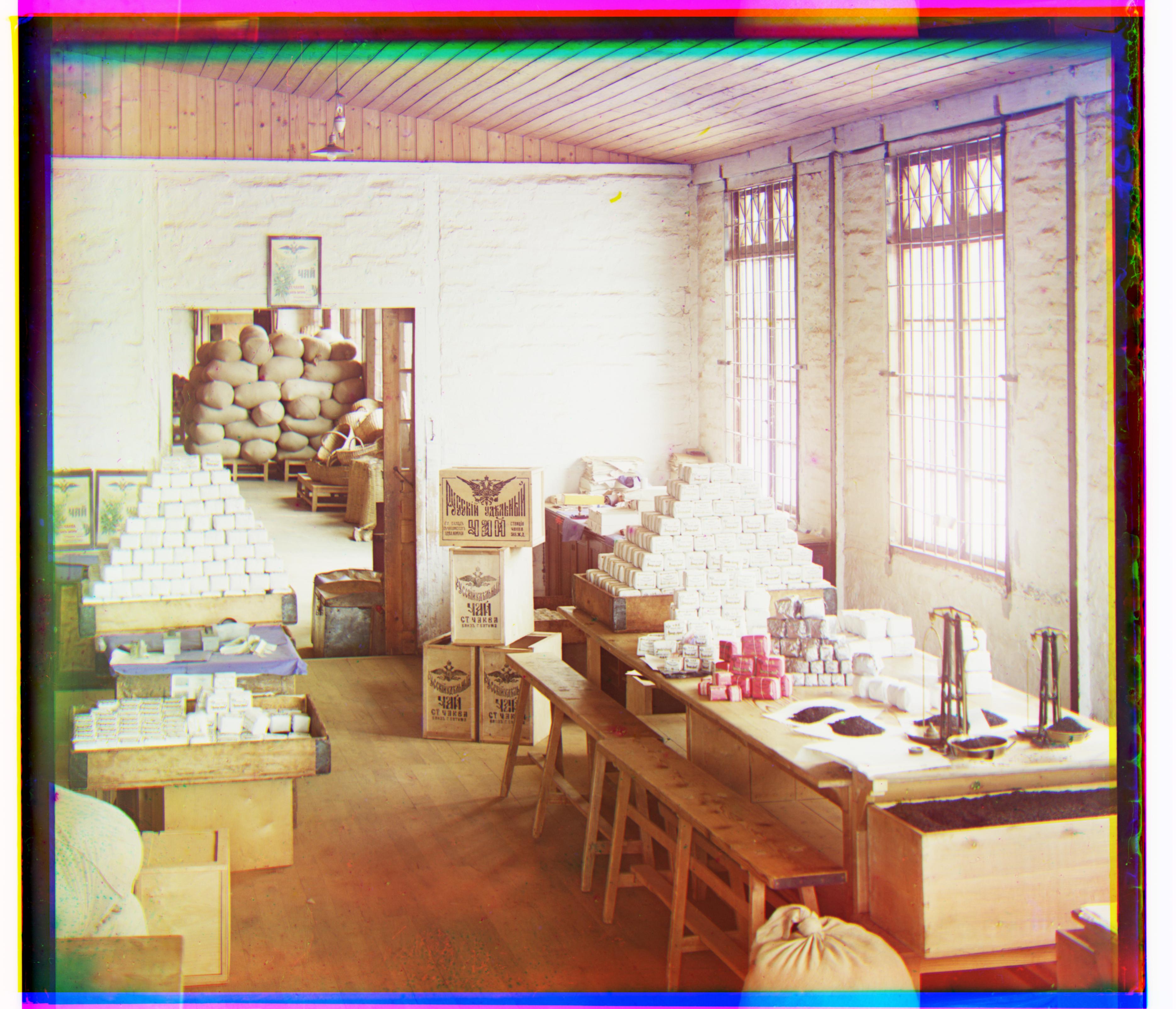
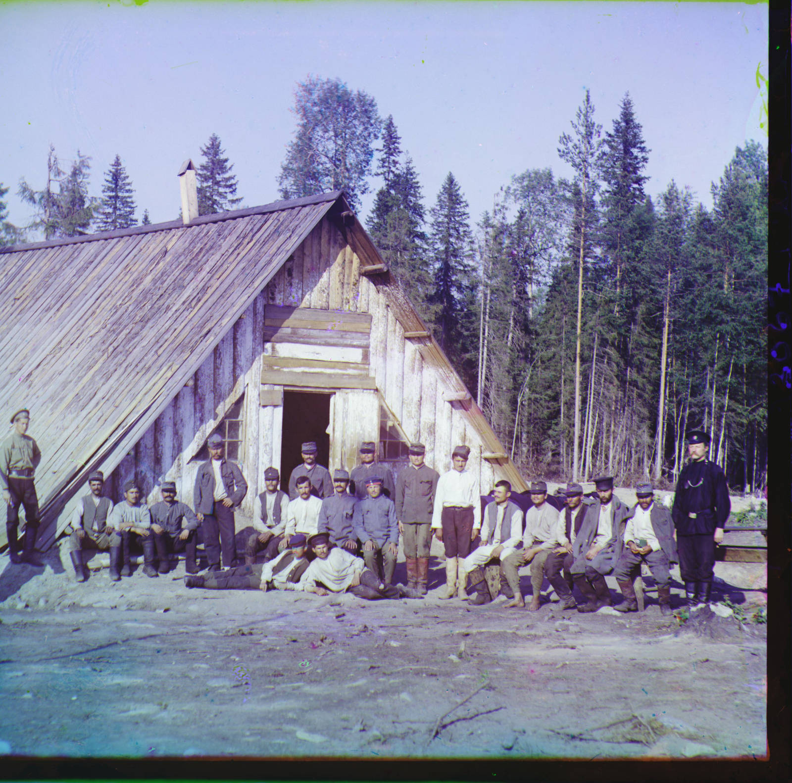
Workshop: ,
Cathedral: ,
Monastery: ,
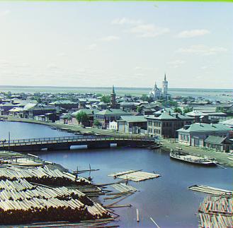
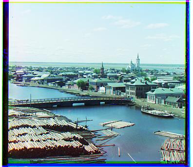
Tobolsk: ,
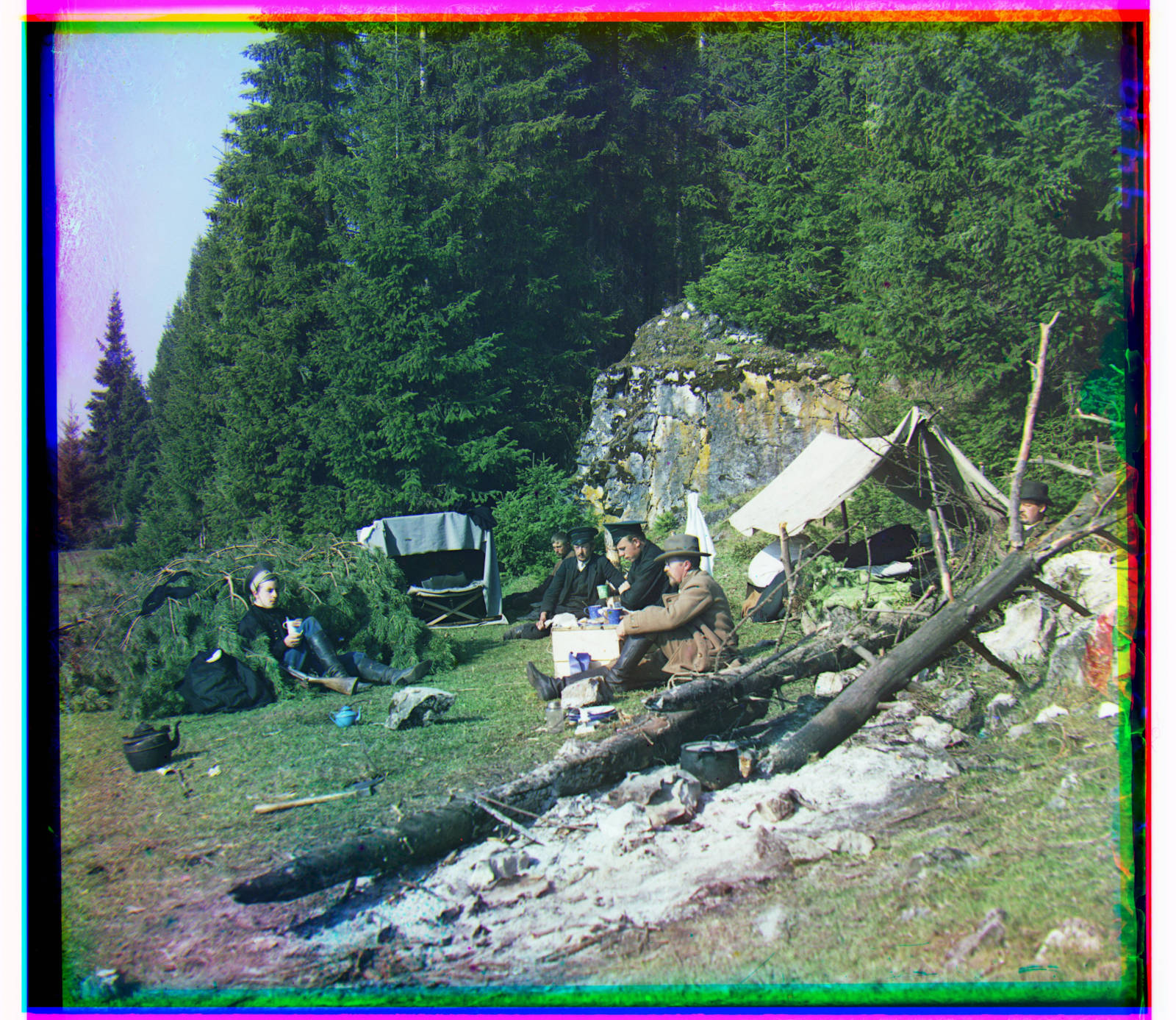
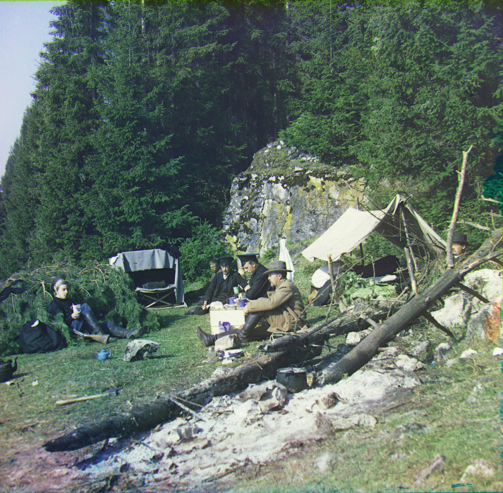
Expedition to the Urals: ,
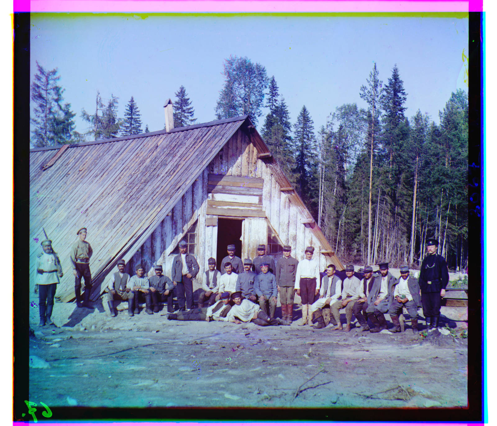
Austro-Hungarian Prisoners of War: ,
Improvements
Similarity metrics
We can observe from the previous results that SSD is not very reliable due to the luminance difference between each channel we are trying to align. Therefore we should introduce a more robust similarity index that tolerates luminance and contrast differences.
The first choice is to instead of using raw pixels, the gradient or edges of the image will be used.
Sobol operator is tested, but this doesn't yeild successful results, as some images may contain much stronger gradients in one color (natural scenes will contain mostly green gradients but none of the red gradients). Therefore, another metric needed to be introduced.
The index of choice here is SSIM (Structural Similarity Index). (https://en.wikipedia.org/wiki/Structural_similarity)
After switching to SSIM, we are able to align all images to a much better precision.
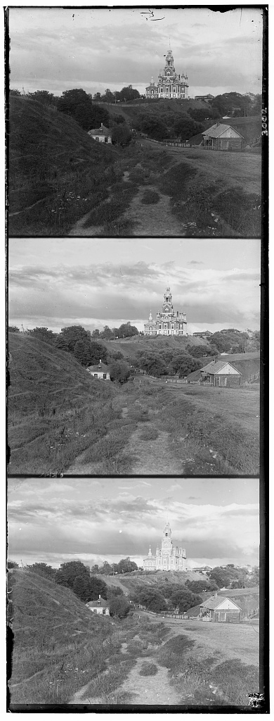
SSD:
SSIM:
Color Correction
Color Mapping
As the original images are captured through colored filter with monochrome glass negatives, the color channel will not map correctly to R, G, B. Color remapping is needed.
The method of color remapping here used is a matrix called Color Correction Matrix. We can multiply this matrix with each color in the aligned output, and therefore remap the color.
The color correction matrix used in this solution is:
Auto White-Balance
The auto white balance algorithm used here is "white patch retinax". This algorithm assumes that there's always a bright patch (spot) in a image, and this spot is perceived as "white". We need to find the brightest spot in the image, and correct that spot to white. This correction is then applied to the whole image.
Auto Dynamic Range
After all these processing, and with the nature of films, the brightest spot and darkest spot are not necessarily white or black. In order to utilize the full range of digital images, the image is remapped to zero to one. The process is achieved by subtracting the whole image by the darkest channel value, and then divided by the brightest channel value. For example, if the darkest color in the image is and the brightest is , the whole image is subtracted by and then divided by .
Auto-cropping
If we start from observing the original data:
We can see that there's a lot of white borders around the image. So the first step is to crop-out the white borders of the image. The aligning process may also shift the image too much to the edge, so before we align the images, we will add a white margin to the R, G, and B images, as the overflowing areas will be cropped later, and it protects the image itself to been cropped.
The detection of white edge is by summing each channel on both X and Y axis:
def cropWhiteEdge(img)
    sumx = average(img over x)
    sumy = average(img over y)

    for v in sumx
        if v > 0.98
            bound = v
        end
    end

    ...
end
If the average brithness on one point on one axis is over , we choose it as one side of the border. This process is repeated for each border on each channel, until we cropped out all the white edges in each image.
After this process, we get a imgage like this:
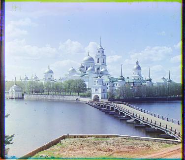
We can observe that there are still colored edges. To detect these edges and crop them out, we will use the cross-channel difference to perform this detection. We compute the summed squared distance of all three channels, then we subtract the average SSD:
Then if the summed error on an edge is greater than , we decide that point on that edge is a border.
After cropping out the colored edges, we get this result:
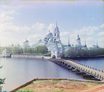
Final Results (after all the bells and whistles)
![]()