import numpy as np
import matplotlib.pyplot as plt
%matplotlib inline
import skimage.io as io
import skimage as sk
from IPython.core.display import HTML
HTML("""
<style>

div.cell { /* Tunes the space between cells */
margin-top:1em;
margin-bottom:1em;
}

div.text_cell_render h1 { /* Main titles bigger, centered */
font-size: 2.2em;
line-height:0.9em;
}

div.text_cell_render h2 { /*  Parts names nearer from text */
margin-bottom: -0.4em;
}


div.text_cell_render { /* Customize text cells */
font-family: 'Georgia';
font-size:1.2em;
line-height:1.4em;
padding-left:3em;
padding-right:3em;
}

.output_png {
    display: table-cell;
    text-align: center;
    vertical-align: middle;
}

</style>

<script>
code_show=true;
function code_toggle() {
 if (code_show){
 $('div.input').hide();
 } else {
 $('div.input').show();
 }
 code_show = !code_show
}
$( document ).ready(code_toggle);
</script>
The raw code for this IPython notebook is by default hidden for easier reading.
To toggle on/off the raw code, click <a href="javascript:code_toggle()">here</a>.

""")
Defining Correspondences
In order to do a face morph, the first step is to define corresponding points on the images and produce a triangulation. I used ginput in order to select 43 points along with 4 points in each fothe corners of the image. For the triangulation, I used the Delaunay triangulation (scipy.spatial.Delaunay) to create triangles between all the corresponding points so an affine transformation can be performed. Below, is the triangulations of my housemate Nolan and I.
im1=plt.imread("dan_triangle.png")
im2=plt.imread("nolan_triangle.png")
fig = plt.figure(figsize=(20,20))
ax1 = fig.add_subplot(1,2,1)
ax1.imshow(im1)
ax1.set_title("Dan")
plt.axis("off")
ax2 = fig.add_subplot(1,2,2)
ax2.imshow(im2)
ax2.set_title("Nolan")
plt.axis("off")
plt.show()

Midway Face
The midway face is the average face shape between my housemate Noland and I. To create the midway face, I first averaged the correspondance points between my face and Nolan's face and found a Delaunay triangulation of those points. Then, for each of the triangles of the average, I use the affine matrix to map the pixels from those triangles to the original image.
im1=plt.imread("daniel.jpg")
im2=plt.imread("midface.jpg")
im3=plt.imread("nolan.jpg")
fig = plt.figure(figsize=(20,20))
ax1 = fig.add_subplot(1,3,1)
ax1.imshow(im1)
ax1.set_title("Dan")
plt.axis("off")
ax2 = fig.add_subplot(1,3,2)
ax2.imshow(im2)
ax2.set_title("Midway Face")
plt.axis("off")
ax3 = fig.add_subplot(1,3,3)
ax3.imshow(im3)
ax3.set_title("Nolan")
plt.axis("off")
plt.show()

Morph Sequence
We had to create a video/gif of 45 frames to create the morph sequence, so I first calculated 45 even points between 0 and 1 (including 0 and 1). Then, for each frame both images were computed similarly to how the midway face was computed except that the warp_factor and dissolve_factor were set to each of those 45 points depending on the frame. I ended up using the same value for the warp_factor and dissolve_factor for each frame.
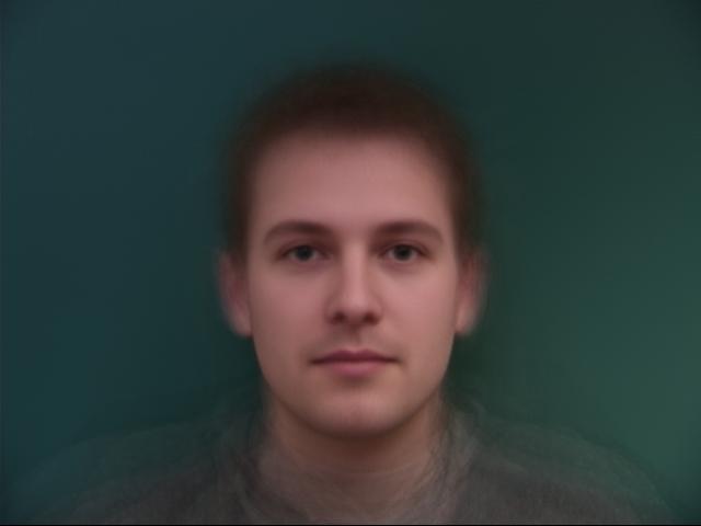
Mean Face of a Population
I found the mean face of the Danes dataset. To do so, I had to first parse the asf files, then load the images and calculate the absolute locations of the correspondance points, compute the average coordinates and traingulate, transform each image to the average coordinates, and then compute the average image. I also computed some of the faces of the Danes morphed to the average face, as well as my face warped into the mean face, and the mean face warped into my face.
Mean face
im1=plt.imread("face_data/01-1m.bmp")
im2=plt.imread("face_data/12-1f.bmp")
im3=plt.imread("face_data/21-1m.bmp")
im4=plt.imread("01-1m-warped.jpg")
im5=plt.imread("12-1f-warped.jpg")
im6=plt.imread("21-1m-warped.jpg")
fig = plt.figure(figsize=(20,10))
ax1 = fig.add_subplot(2,3,1)
ax1.imshow(im1)
ax1.set_title("01")
plt.axis("off")
ax2 = fig.add_subplot(2,3,2)
ax2.imshow(im2)
ax2.set_title("12")
plt.axis("off")
ax3 = fig.add_subplot(2,3,3)
ax3.imshow(im3)
ax3.set_title("21")
plt.axis("off")
ax4 = fig.add_subplot(2,3,4)
ax4.imshow(im4)
ax4.set_title("01 warped")
plt.axis("off")
ax5= fig.add_subplot(2,3,5)
ax5.imshow(im5)
ax5.set_title("12 warped")
plt.axis("off")
ax6 = fig.add_subplot(2,3,6)
ax6.imshow(im6)
ax6.set_title("21 warped")
plt.axis("off")
plt.show()

im1=plt.imread("dan_dutch.jpg")
im2=plt.imread("dutch_dan.jpg")
fig = plt.figure(figsize=(20,20))
ax1 = fig.add_subplot(1,2,1)
ax1.imshow(im1)
ax1.set_title("Dutch Dan")
plt.axis("off")
ax2 = fig.add_subplot(1,2,2)
ax2.imshow(im2)
ax2.set_title("Dan Dutch")
plt.axis("off")
plt.show()

Caricatures: Extrapolating from the Mean
The above warped images are computed with the following formula, N = A (1-$\alpha$) + B($\alpha$) where $\alpha \in [0,1]$. However, we can extrapolate from the mean by using $\alpha$ beyond this range. This will create "Caricatures", where the face is morphed more than expected.
im1=plt.imread("caricature_dan1.jpg")
im2=plt.imread("caricature_dan2.jpg")
fig = plt.figure(figsize=(20,20))
ax1 = fig.add_subplot(1,2,1)
ax1.imshow(im1)
ax1.set_title("alpha = 2")
plt.axis("off")
ax2 = fig.add_subplot(1,2,2)
ax2.imshow(im2)
ax2.set_title("alpha = -3")
plt.axis("off")
plt.show()

Bells and Whistles: Changing my expression
My face is pretty neutral in my picture, and decided to try to make myself smile. I decided to use the Danes data again to do so, as there is a picture for each person that's smiling. I computed the mean smiling face, and created images where I only change the only the shape (morphing), appearance (color), and both the appearance and shape of my face. Using only the shape warps my face into a smile, but warps my glasses/upper face as well. Using only the appearance adds some of the shadows from smiling, noticible in the cheek area, and adding both accentuates both effects.
im1=plt.imread("daniel_new.jpg")
im2=plt.imread("smile_dan_shape.jpg")
im3=plt.imread("smile_dan_color.jpg")
im4=plt.imread("smile_dan.jpg")
fig = plt.figure(figsize=(40,20))
ax1 = fig.add_subplot(1,4,1)
ax1.imshow(im1)
ax1.set_title("Dan")
plt.axis("off")
ax2 = fig.add_subplot(1,4,2)
ax2.imshow(im2)
ax2.set_title("Dan warped")
plt.axis("off")
ax3 = fig.add_subplot(1,4,3)
ax3.imshow(im3)
ax3.set_title("Dan with color")
plt.axis("off")
ax4 = fig.add_subplot(1,4,4)
ax4.imshow(im4)
ax4.set_title("Dan warped + colored")
plt.axis("off")
plt.show()
