
by Suraj Rampure (suraj.rampure@berkeley.edu, cs194-26-adz)
Here, we use triangulations to create morphs between images.
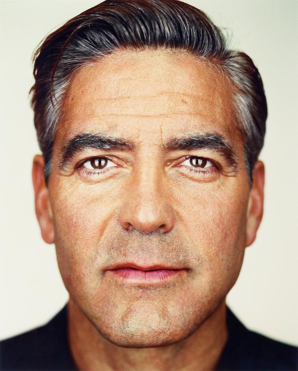
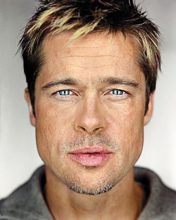
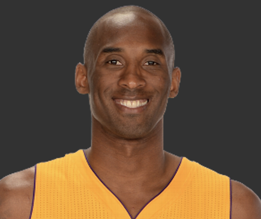
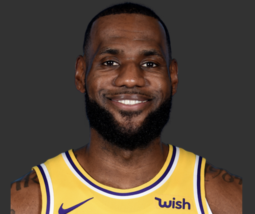
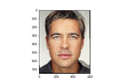
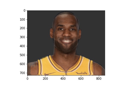
For the first three parts – “Defining Correspondences”, “Computing the Mid-Way Face”, and “The Morph Sequence”, I did everything on two pairs of images. The first pair is of George Clooney and Brad Pitt, and the second is of Kobe Bryant (RIP) and LeBron James.
Pair 1:
Pair 2:
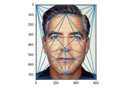
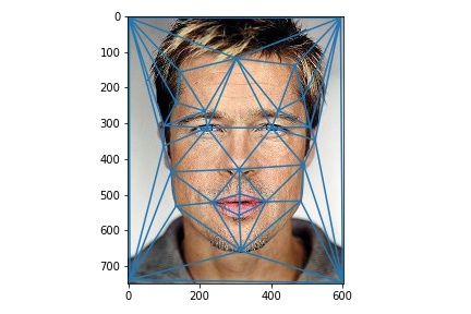
First, we use ginput to select key points on each image – roughly 30 of them. Then, we take the average of these key points, and create a triangulation out of them. To do this, I used scipy.signal.Delaunay, generating a Delaunay triangulation as specified in class.
Triangulation on Pair 1:
Triangulation on Pair 2:
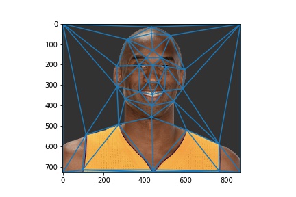
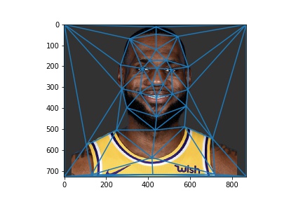
Note: Since we apply the same triangulation to both images in a pair, the triangulations are topologically the same. (We do this by calling Delauney(average_key_points).simplices); the simplices attribute gives an ordering of the key points.)
Now, I implemented compute_affine(t1, t2), as indicated in the spec. This returns a 3x3 matrix, that allows us to take an [x, y, 1] coordinate in triangle t1 and map it to [x', y', 1] in triangle t2.
In order to compute the half-way face, I applied this transformation to each triangle in the triangulation of the average of the key points. Specifically, for each triangle, I extracted the relevant region from the “left” and “right” images, and multiplied both regions by 0.5 to create a true middle half-way face (resulting in the average of both the spatial features and the colors).
Half-way images of Pair 1 and Pair 2:
The George-Brad half-way face looks a little more realistic, since their faces were in the exact same position and are of the exact same size. Since you can see LeBron’s beard in the LeBron-Kobe half-way face, that half-way image looks a little more like LeBron (but you can see Kobe’s eyes and jersey).
Then, as required, I implemented the morph(im1, im2, im1_pts, im2_pts, tri, f) function, that takes in two images, their key points, a triangulation, and a fraction f, and computes the image f of the way between image 1 and image 2 (that is, if f = 0, this just returns image 1). The only change from above was instead of just averaging the key points of the two images, I weighed them as (1-f) * im1_pts + f * im2_pts (this is the behavior of warp_frac); similarly, instead of averaging the extracted regions of both images, I weighed them by 1-f and f (the behavior of dissolve_frac). I saw no need to have two separate fractions.
I let f take on values in [0, 1/45, 2/45, 3/45, ..., 44/45, 45/45], creating a 45 (well, 46) frame animation. The gifs of the morph between the left and right images for both pairs are shown here (they might take a while to load since I had to host them on some random website because of file size constraints):
Pair 1:

Pair 2:
For the Kobe-LeBron hybrid, the face morph works a lot better than the jersey morph, since the older and newer jerseys aren’t really the same structurally.
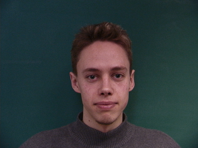
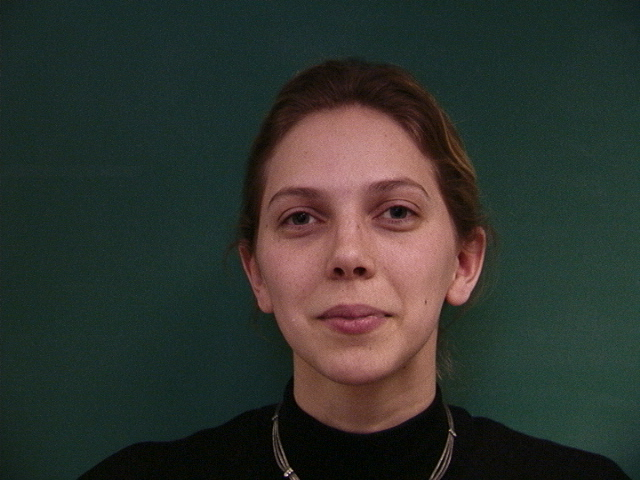
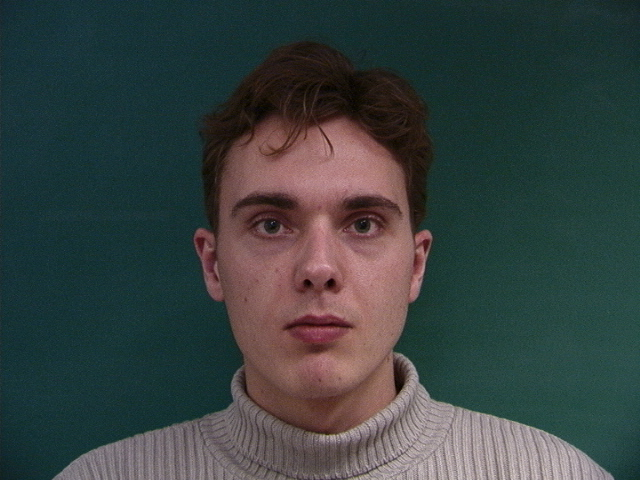
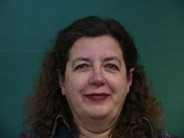
For this portion of the assignment, I used the dataset of images of Danish computer scientists that was linked in the project spec. I computed the mean face of all 37 Danes; in order to do this, I tweaked my work from earlier that averaged 2 images to instead average all 37 (both spatially and in the color space).
Here are some of those Danes, for context:
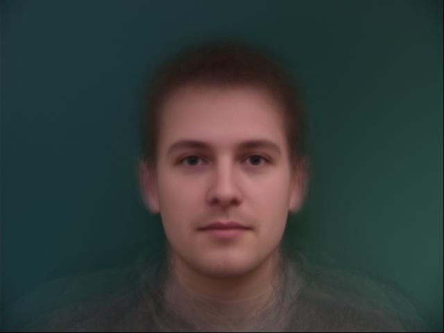
Here’s the result – not so mean looking!
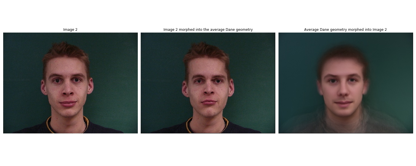
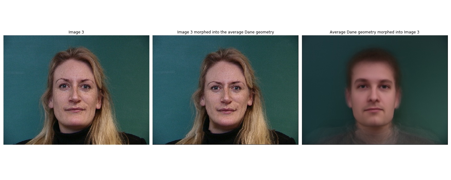
I then morphed some of the faces into the average geometry of the Danes faces’ (i.e. the geometry of the image above), as well as the average face into the geometry of the selected images. Here are the results:
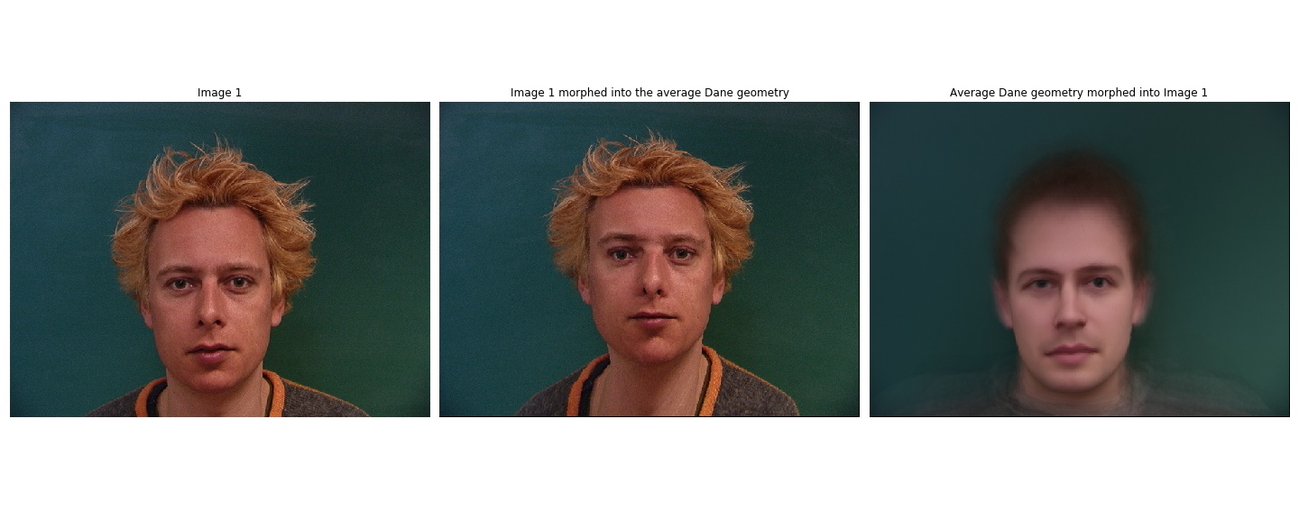
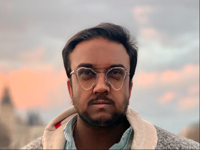
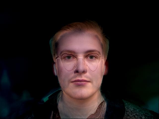
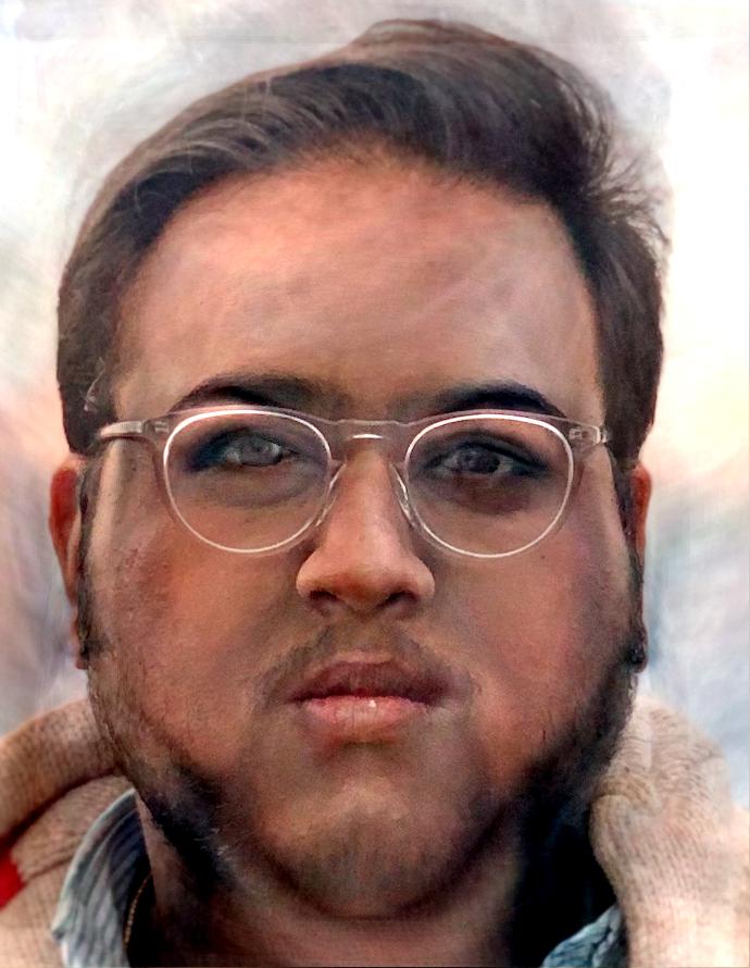
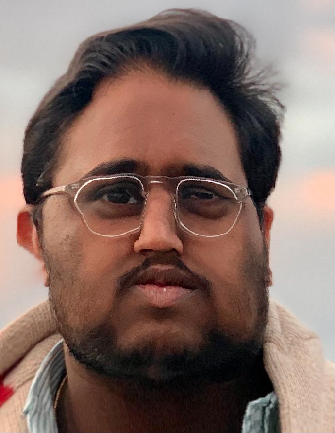
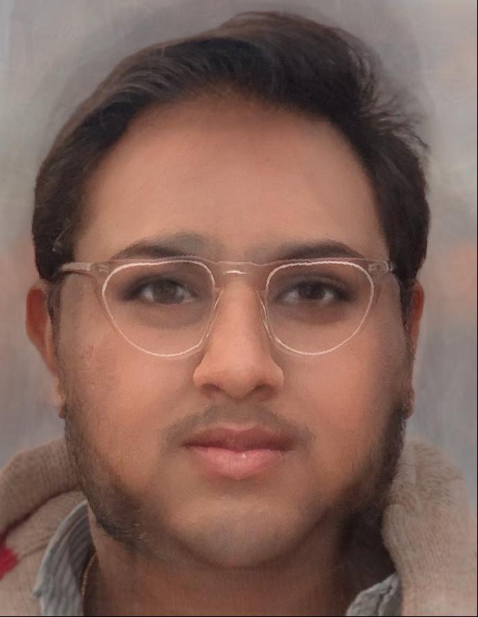
I also took the following image of myself:
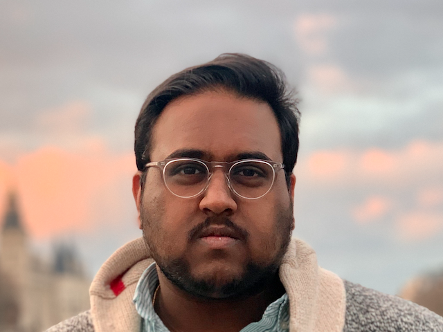
and both 1. morphed it into the average geometry of the Danes, and 2. morphed the average Dane into the geometry of me. This required annotating the image of my face in the exact same way that the Danes’ faces were annotated; I referred to the report linked at the site above to do so. Here are the results:
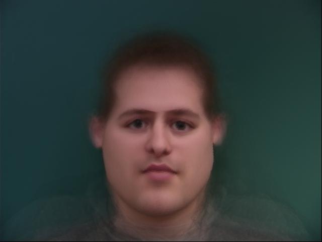
While the latter is not great for my self-esteem, at least I know my code works! 🥺
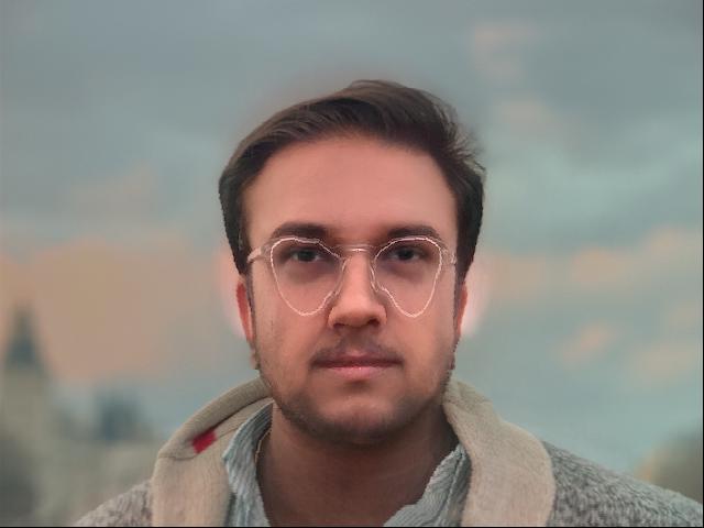
Using the following expression, I then computed caricatures of my face within the subspace of the average Dane image:
(mean_dane + (me_to_dane - mean_dane) * alpha)
where me_to_dane is the image of me in the geometry of the average Dane (the image on the left above). Here are the results when using alpha = -0.5, alpha = 0.5, and alpha = 1.5 respectively:
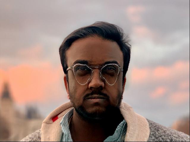
For this, I used the images on this site to morph my face into the average Bollywood actress. To do this, I used the following images of the average Bollywood male actor and average Bollywood female actress:
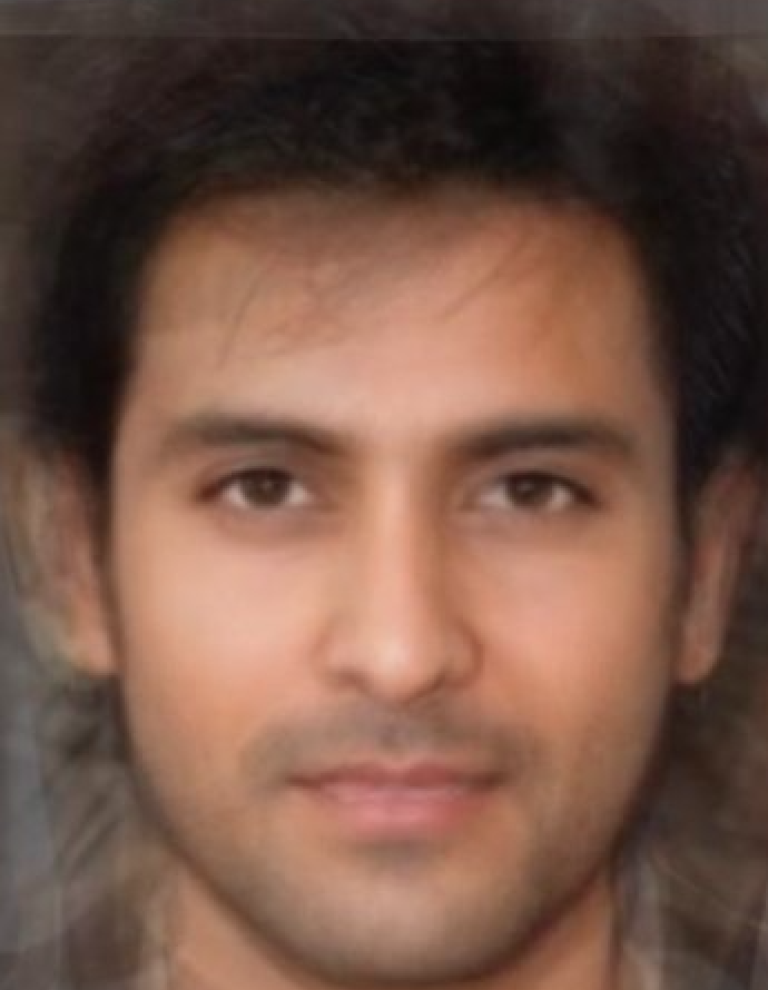
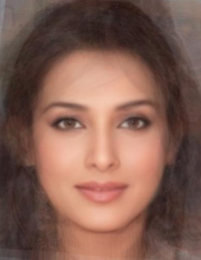
Each of the following morphs rely on adding the difference between the average Bollywood female’s face and the average Bollywood male’s face to my face. They don’t turn out that great, because, well, I don’t quite look like a Bollywood actor.
Here’s the result when computing an appearance-only morph (attained by spatially morphing both the female and male images to that of me, and then adding the difference of these two morphed images to my original image):
Here’s the shape-only morph:
And finally, the total morph:
This was a super cool project. As the semester progresses, it’s been eye-opening to see how many of the Snapchat / Instagram effects that have become so commonplace can all be implemented using not-so-complicated math.