from IPython.core.display import HTML
HTML("""
<style>
div.cell { /* Tunes the space between cells */
margin-top:1em;
margin-bottom:1em;
}
div.text_cell_render h1 { /* Main titles bigger, centered */
font-size: 2.2em;
line-height:0.9em;
}
div.text_cell_render h2 { /* Parts names nearer from text */
margin-bottom: -0.4em;
}
div.text_cell_render { /* Customize text cells */
font-family: 'Georgia';
font-size:1.2em;
line-height:1.4em;
padding-left:3em;
padding-right:3em;
}
.output_png {
display: table-cell;
text-align: center;
vertical-align: middle;
}
</style>
<script>
code_show=true;
function code_toggle() {
if (code_show){
$('div.input').hide();
} else {
$('div.input').show();
}
code_show = !code_show
}
$( document ).ready(code_toggle);
</script>
<!---The raw code for this IPython notebook is by default hidden for easier reading.
To toggle on/off the raw code, click <a href="javascript:code_toggle()">here</a>.--->
""")
from IPython.display import HTML
HTML('''<script>
code_show_err=true;
function code_toggle_err() {
if (code_show_err){
$('div.output_stderr').hide();
} else {
$('div.output_stderr').show();
}
code_show_err = !code_show_err
}
$( document ).ready(code_toggle_err);
</script>''')
Defining Correspondences
Before we can begin to morph faces together, we need to define points on each face that we can use to map one face to another. In order to select points on two images simultaneously, I wrote a separate python script - gen_points.py. In it, I use matplotlib's ginput to manually select points on the two faces. I chose these points to be key features of each face (e.g. eyes, lips, ears, chin, etc.). The script then wrote these points to disk in the form of a .npy file that I read into my notebook and used there on out.
Once the point correspondences were defined, the next step was to define a triangulation of the image on said points. This was done to segment our image into many triangles - triangles that would then be used in a local warp to morph the images. For this project we used the Delaunay triangulation because it maximizes the smallest angles of the triangles and thus gives us more evenly sized triangles. Since we only want one triangulation to morph between images, I arbitrarily picked my first image, constructed the triangulation on that, and used that for both images.
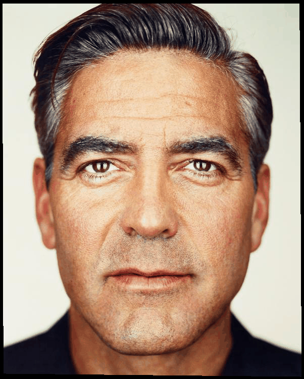
The two images I used were the provided image of George Clooney and an image of his frequent co-star Brad Pitt. Below are the two images with their correspondences and triangulations overlayed.
import numpy as np
import matplotlib.pyplot as plt
from scipy.spatial import Delaunay
from skimage.draw import polygon
from skimage.util import img_as_float
import imageio
import glob
from sklearn.decomposition import PCA
george = plt.imread("data/george.jpg")
brad = plt.imread("data/brad.jpg")
george_pts = np.load("out/george.npy")
brad_pts = np.load("out/brad.npy")
tri = Delaunay(george_pts)
plt.figure(figsize=(15,10))
plt.subplot(121)
plt.imshow(george)
plt.scatter(*zip(*george_pts))
plt.triplot(george_pts[:,0], george_pts[:,1], tri.simplices)
plt.axis("off")
plt.subplot(122)
plt.imshow(brad)
plt.scatter(*zip(*brad_pts))
plt.triplot(brad_pts[:,0], brad_pts[:,1], tri.simplices)
plt.axis("off")
plt.show()

Computing the "Mid-way Face"
Before creating the full morph sequence, I computed the mid-way face of the two images. This process involved three steps:
- Creating an average shape, or average of the keypoint correspondences
- Warping both faces into the created average shape
- Blending the colors of each image together
The main step of this process was the actual warping of faces to the average shape. This was implemented by calculating an affine mapping between each triangle in the triangulation of each image to the mid-way triangulation. The set of these transformation matrices was then used to implement an inverse warp to morph the images into the mid-way face. I did not end up using any interpolation (other than rounding the co-ordinates) as it was the quickest option (computationally) and still had good results.
The two images and the mid-way face are shown below.
mid_pts = np.mean(np.stack((george_pts, brad_pts)), axis=0)
def compute_affine(tri1_pts, tri2_pts):
#Creates a mapping from tr1 to tri2 - tri2 should be destination
dest = np.concatenate((tri2_pts.flatten(),np.ones(1)))[:,None] # Creating (7,1) vector
tri1_pts = np.hstack((tri1_pts, np.ones((3,1)))) #Adding fictitious 1 dimension
# Bunch of code to create my 7x7 matrix mat
test3 = np.hstack((tri1_pts, np.zeros((3,3))))
test4 = np.hstack((np.zeros((3,3)), tri1_pts))
test5 = np.array(np.vstack(zip(test3, test4)))
mat = np.zeros((7,7))
mat[:6,:6] = test5
mat[-1,-1] = 1
res = np.linalg.inv(mat).dot(dest)
res = res[:-1].reshape(2,3) #getting rid of fictitious dimension
transform = np.zeros((3,3))
transform[:2, :3] = res
transform[-1,-1] = 1
return transform
mid_triangles = mid_pts[tri.simplices]
george_triangles = george_pts[tri.simplices]
brad_triangles = brad_pts[tri.simplices]
mid_im = np.zeros_like(george)
for i, triangles in enumerate(zip(mid_triangles, george_triangles, brad_triangles)):
mid_tri, george_tri, brad_tri = triangles
T1 = compute_affine(mid_tri, george_tri)
T2 = compute_affine(mid_tri, brad_tri)
cc, rr = polygon(mid_tri[:,0],mid_tri[:,1])
poly_arr = np.array((cc, rr))
mid_domain = np.vstack((poly_arr, np.ones((1, poly_arr.shape[1]))))
george_domain = np.round(T1.dot(mid_domain)[:2,:]).astype(int)
brad_domain = np.round(T2.dot(mid_domain)[:2,:]).astype(int)
g_pix = george[george_domain[1,:], george_domain[0,:]].astype(float)
b_pix = brad[brad_domain[1,:], brad_domain[0,:]].astype(float)
mid_im[rr,cc] = 0.5*(g_pix+b_pix)
plt.figure(figsize=(15,10))
plt.subplot(131)
plt.imshow(george)
plt.title("George Clooney")
plt.axis("off")
plt.subplot(132)
plt.imshow(brad)
plt.title("Brad Pitt")
plt.axis("off")
plt.subplot(133)
plt.imshow(mid_im)
plt.title("George Pitt? Brad Clooney? (Mid-Way Face)")
plt.axis("off")
plt.show()

The Morph Sequence
The same procedure that was used to create a mid-way face was repeated several times to create the morph sequence. Rather than taking the midpoint (or the average), I took the weighted average (parameterized by $t$) of both the keypoints and the colors, and repeated this for $45$ evenly spaced values of $t\in[0,1]$. The resulting image volume was then written as a gif to disk and displayed below.
def morph(im1, im2, im1_pts, im2_pts, tri, warp_frac):
im1_triangles = im1_pts[tri.simplices]
im2_triangles = im2_pts[tri.simplices]
out = np.zeros((int(1/warp_frac)+1, *im1.shape))
# print(out.shape)
for idx, t in enumerate(np.arange(0, 1+warp_frac, warp_frac)):
intermediate_pts = (1-t)*im1_pts+t*im2_pts
intermediate_triangles = intermediate_pts[tri.simplices]
intermediate_im = np.zeros_like(im1)
for i, triangles in enumerate(zip(intermediate_triangles, im1_triangles, im2_triangles)):
intermediate_tri, im1_tri, im2_tri = triangles
T1 = compute_affine(intermediate_tri, im1_tri)
T2 = compute_affine(intermediate_tri, im2_tri)
cc, rr = polygon(intermediate_tri[:,0],intermediate_tri[:,1])
poly_arr = np.array((cc, rr))
intermediate_domain = np.vstack((poly_arr, np.ones((1, poly_arr.shape[1]))))
im1_domain = np.round(T1.dot(intermediate_domain)[:2,:]).astype(int)
im2_domain = np.round(T2.dot(intermediate_domain)[:2,:]).astype(int)
pix_1 = im1[im1_domain[1,:], im1_domain[0,:]].astype(float)
pix_2 = im2[im2_domain[1,:], im2_domain[0,:]].astype(float)
intermediate_im[rr,cc] = (1-t)*pix_1+t*pix_2
# plt.imsave("out/morph_{}.jpg".format(int(t/warp_frac)), intermediate_im)
# print(int(t/warp_frac))
out[idx] = intermediate_im
return out
out = morph(george, brad, george_pts, brad_pts, tri, 1/45)
# Saving gif to disk
# images = [img for img in out]
# imageio.mimsave('out/morph.gif', images)
The "Mean Face" and Caricatures of a Population
Using the Dane dataset, I created the "Mean Face" of that dataset. This was done by finding the average shape (average of keypoints), morphing every image into that shape, and then averaging all the morphed images.
One note is that I had to slightly augment the keypoints in the dataset to include the four corners of the image. As given, the correspondences only covered the facial region, so adding the four corners gave the resulting mean image a background.
I also created a caricature image by morphing the average image into specific people's facial geometry. The results are shown and labeled below.
fnames = sorted(glob.glob("data/face_db/*.bmp"))
dane_ims = []
for fname in fnames:
dane_ims.append(plt.imread(fname))
# print(*list(zip(sorted(glob.glob("data/face_db/*.asf")),sorted(glob.glob("data/face_db/*.bmp")))), sep="\n")
fnames = sorted(glob.glob("data/face_db/*.asf"))
data_pt_list = []
for i, fname in enumerate(fnames):
with open(fname) as f:
data = f.readlines()[16:-5]
pts = [data[i].split("\t")[2:4] for i in range(len(data))]
dims = dane_ims[i].shape
pts = np.stack([np.array([float(pt[0])*dims[1], float(pt[1])*dims[0]]) for pt in pts])
pts = np.vstack((pts, np.array([[1, 1], [dims[1]-1, 1], [1, dims[0]-1], [dims[1]-1, dims[0]-1]])))
data_pt_list.append(pts)
dane_tri = Delaunay(data_pt_list[0])
mean_pts = np.mean(np.stack(data_pt_list), axis=0)
plt.figure(figsize=(15,10))
plt.imshow(dane_ims[0])
plt.scatter(*zip(*data_pt_list[0]))
plt.triplot(data_pt_list[0][:,0], data_pt_list[0][:,1], dane_tri.simplices)
plt.title("Example data from dataset")
plt.axis("off")
plt.show()

def morph_shape(start_im, start_shape, goal_shape, tri):
mid_triangles = goal_shape[tri.simplices]
dat_triangles = start_shape[tri.simplices]
morphed_im = np.zeros_like(start_im)
for i, triangles in enumerate(zip(mid_triangles, dat_triangles)):
mid_tri, dat_tri = triangles
T = compute_affine(mid_tri, dat_tri)
cc, rr = polygon(mid_tri[:,0],mid_tri[:,1])
poly_arr = np.array((cc, rr))
mid_domain = np.vstack((poly_arr, np.ones((1, poly_arr.shape[1]))))
morphed_domain = np.round(T.dot(mid_domain)[:2,:]).astype(int)
morphed_im[rr,cc] = start_im[morphed_domain[1,:], morphed_domain[0,:]].astype(float)
return morphed_im
# mid_triangles = mean_pts[dane_tri.simplices]
morphed_ims = []
for idx, dat in enumerate(data_pt_list):
morphed_im = morph_shape(dane_ims[idx], dat, mean_pts, dane_tri)
morphed_ims.append(morphed_im)
face_stack = img_as_float(np.stack(morphed_ims))
avg_face = np.mean(face_stack, axis=0)
titles = ["Original Danes","Morphed to Mean"]
imgs = dane_ims[:3]+list(face_stack[:3])
fig, axs = plt.subplots(2, 3, figsize=(20, 10))
for i, ax in enumerate(axs.flatten()):
ax.imshow(imgs[i])
# ax.axis("off")
ax.get_xaxis().set_visible(False)
ax.get_yaxis().set_ticks([])
for ax, row in zip(axs[:,0], titles):
ax.set_ylabel(row, rotation=90, fontsize=16)
fig.tight_layout()
plt.show()

plt.figure(figsize=(15,10))
plt.imshow(avg_face)
plt.title("Mean Face")
plt.axis("off")
plt.show()

idx = 10
plt.figure(figsize=(15,10))
plt.imshow(morph_shape(avg_face, mean_pts, data_pt_list[idx], dane_tri))
plt.title("Caricature - mean face morphed to an indiviual's shape")
plt.axis("off")
plt.show()

Bells and Whistles - Using PCA to create Caricatures
As a Bells and Whistles, I decided to use PCA to create caricatures. This was done by treating each image as a vector and running PCA on the resultant data matrix. I then took the mean image and added a proportional amount of each singular vector to it to create a caricature. The results are shown below.
N_EIGEN_FACES = 15
data_matrix = face_stack.reshape(37,-1)
IMG_SHAPE = face_stack[0].shape
pca = PCA(n_components=N_EIGEN_FACES)
pca.fit(data_matrix)
mean = pca.mean_
eigenvectors = pca.components_.tolist()
eigenvectors = [np.asarray(eigenvectors[i]) for i in range(len(eigenvectors))]
mean_face = mean.reshape(IMG_SHAPE)
mean_face = np.asarray(mean_face)
slider_values = []
eigen_faces = []
for eigenvector in eigenvectors:
tmp_face = eigenvector.reshape(IMG_SHAPE)
eigen_faces.append(tmp_face)
def make_face(*args):
new_face = mean_face
for i in range(N_EIGEN_FACES):
slider_values[i] = cv2.getTrackbarPos("Weight" + str(i), "Trackbars")
weight = slider_values[i] - MAX_SLIDER_VALUE/2
new_face = new_face + eigen_faces[i]*weight*100
new_face = np.maximum(np.minimum(new_face, 255),0)
new_face = np.asarray(new_face, dtype=np.uint8)
cv2.imshow("Demo face", new_face)
plt.figure(figsize=(15,10))
plt.imshow(mean_face)
plt.title("Mean Face (from PCA analysis)")
plt.axis("off")
plt.show()

# plt.figure(figsize=(25,15))
# for i, eface in enumerate(eigen_faces):
# plt.subplot(3, 5, i+1)
# plt.imshow(mean_face+eface*100)
# plt.axis("off")
# plt.title("Mean + Singular Vec_{}".format(i+1))
# titles = ["Original Danes","Morphed to Mean"]
# imgs = dane_ims[:3]+list(face_stack[:3])
fig, axs = plt.subplots(5, 3, figsize=(15, 25))
for i, ax in enumerate(axs.flatten()):
ax.imshow(mean_face+110*eigen_faces[i])
ax.set_title("Mean + Singular_Vec_{}".format(i+1), fontsize=16)
ax.axis("off")
# ax.get_xaxis().set_visible(False)
# ax.get_yaxis().set_ticks([])
# for ax, row in zip(axs[:,0], titles):
# ax.set_ylabel(row, rotation=90, fontsize=16)
fig.tight_layout()
plt.show()
