Classification and Segmentation
Chris Mitchell
Overview
For this project I applied pytorch to the computer vision problems of classification and segmentation.
Classification
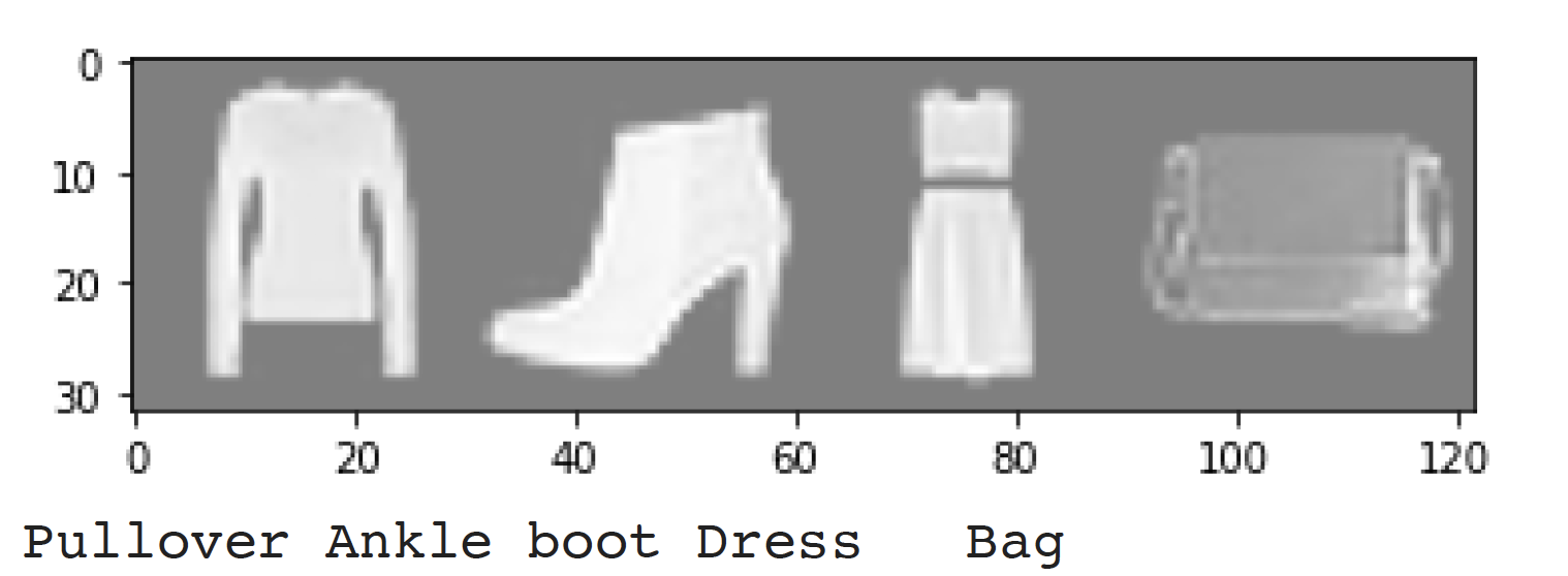
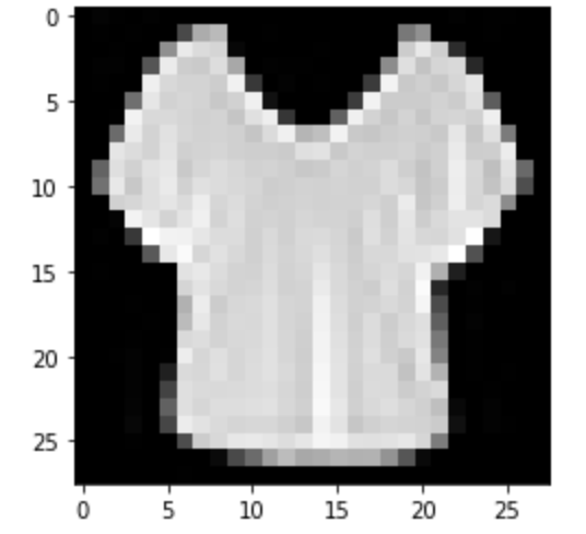
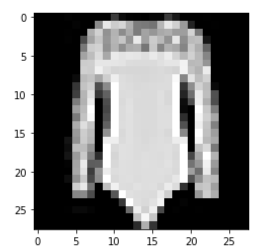
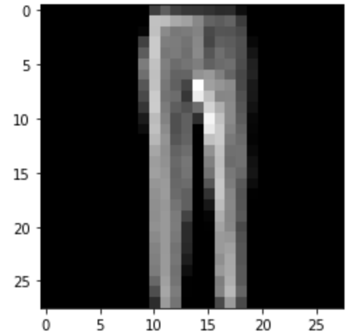
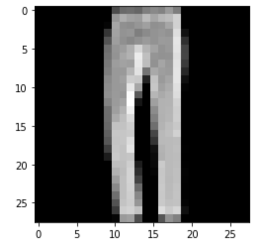
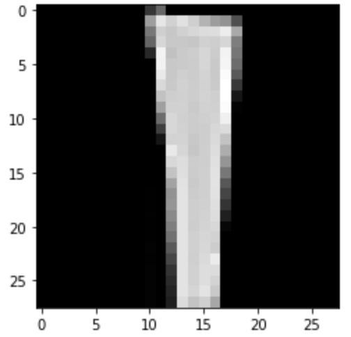
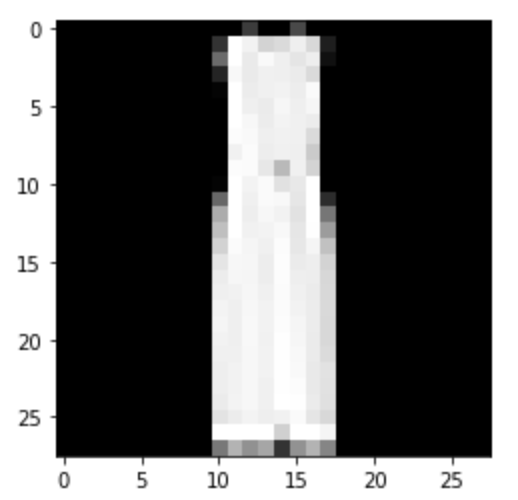
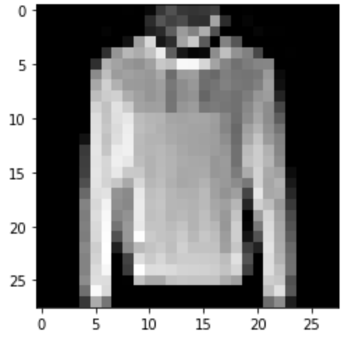
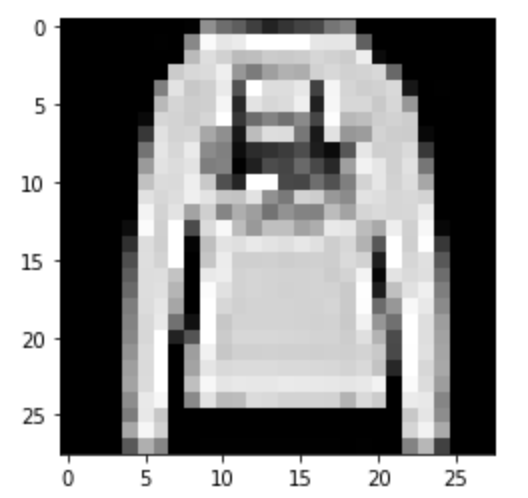
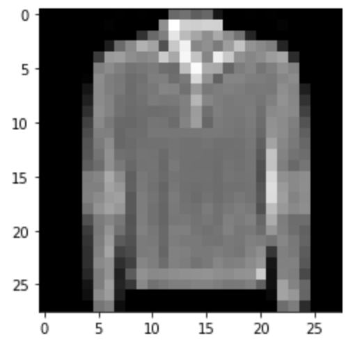
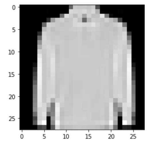
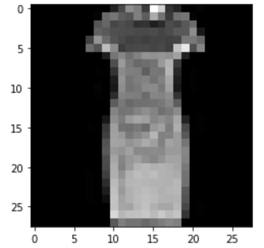
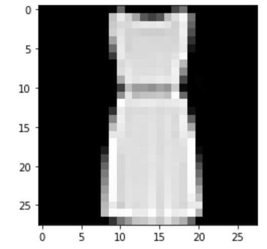
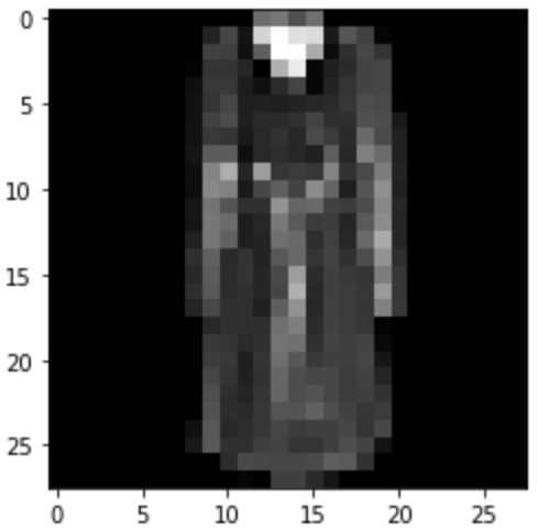
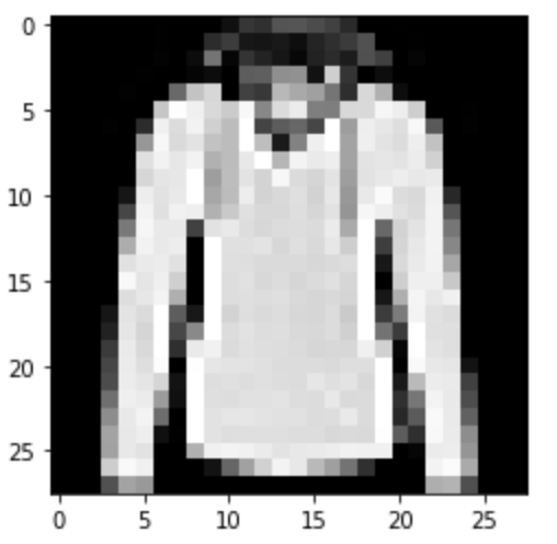
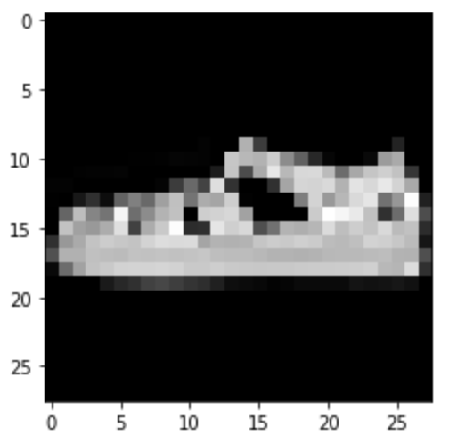
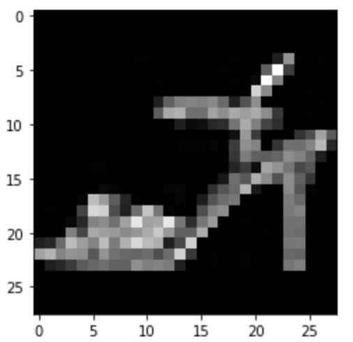
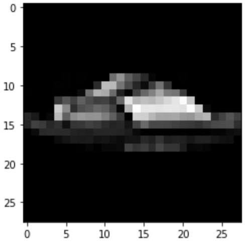
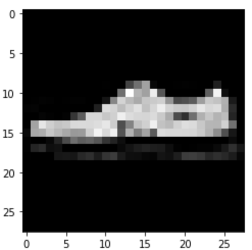
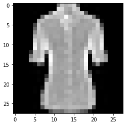
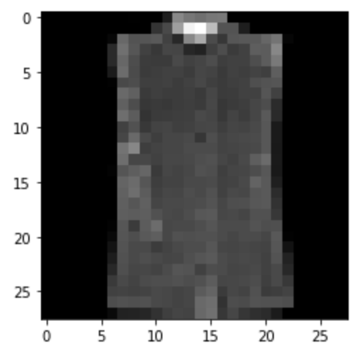
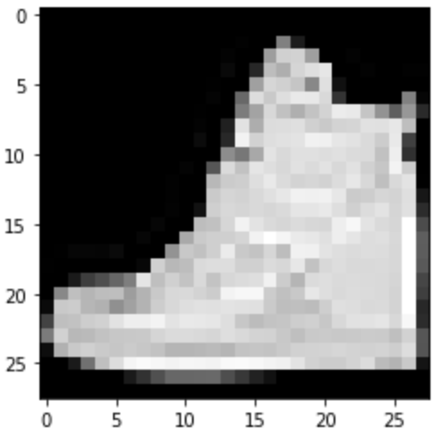
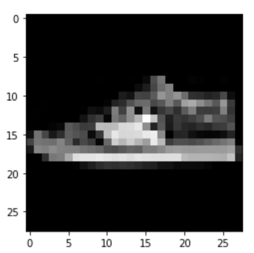
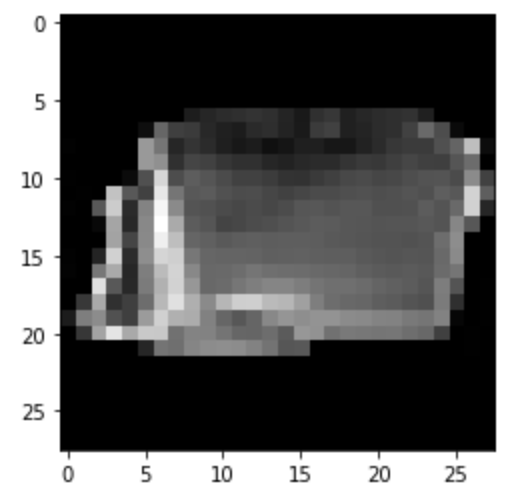
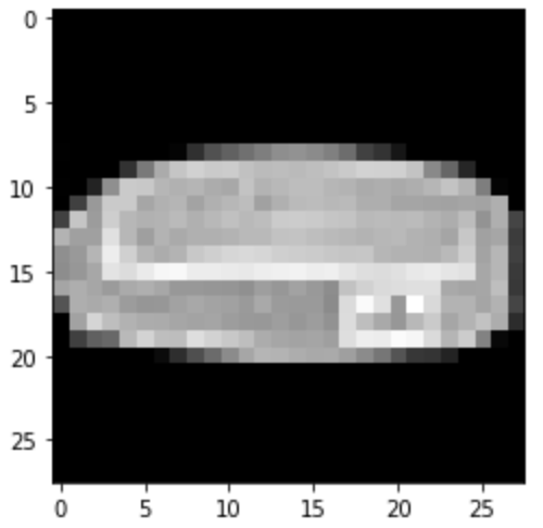
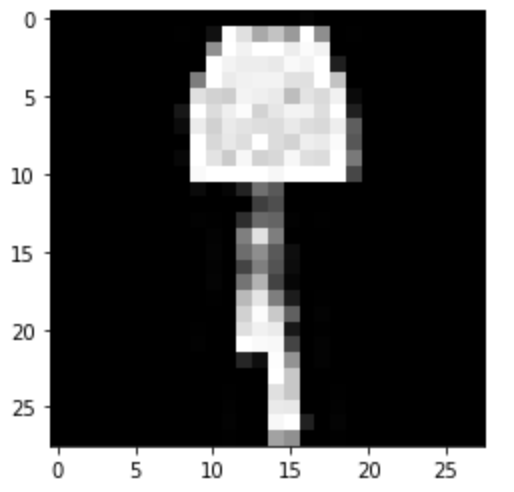
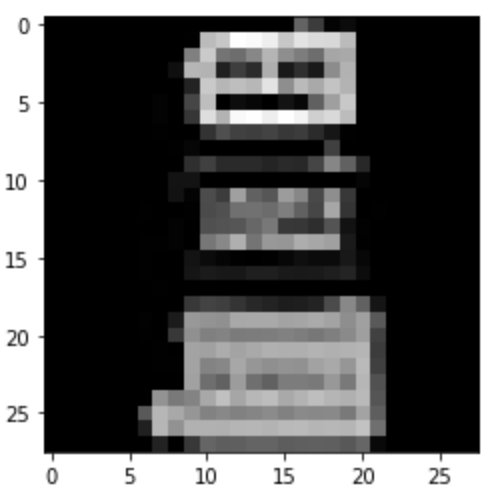
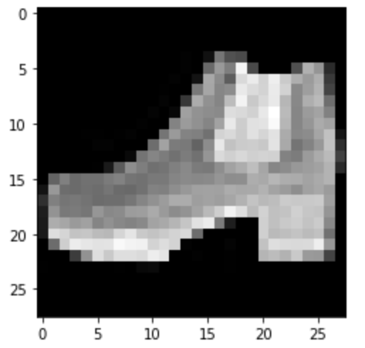
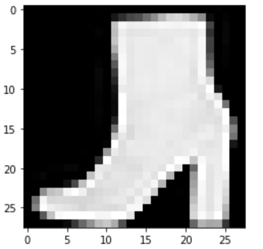
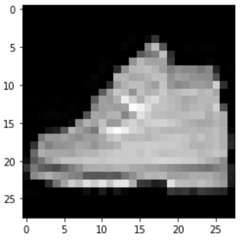
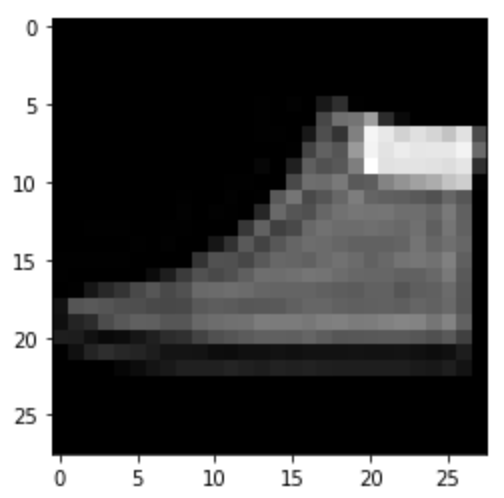
Using the Fashion MNIST dataset, I trained a neural network to classify the clothing images into their different types
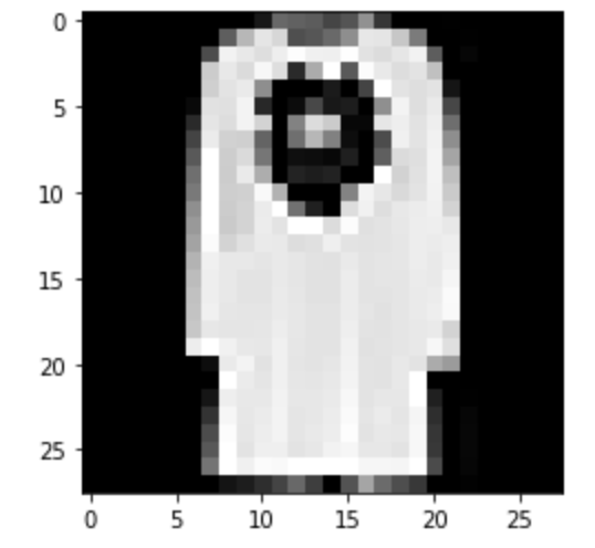
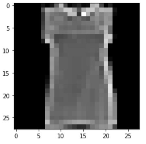
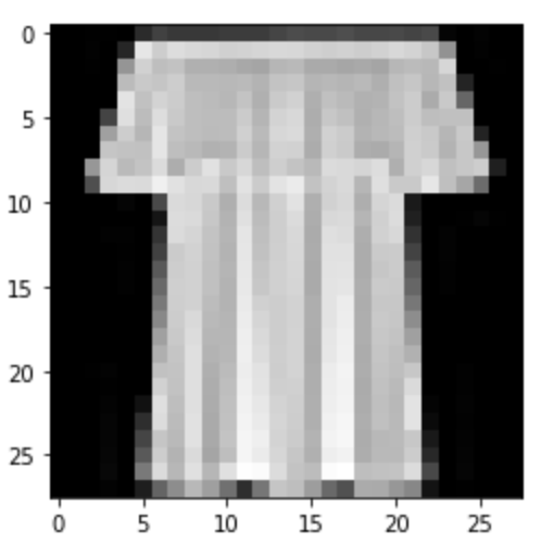
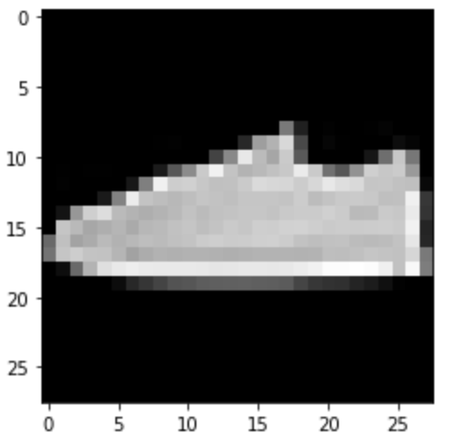
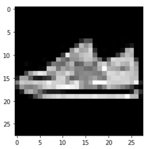
Data from the Fashion MNIST dataset
For this neural network, I had two layers of convolution and max pooling followed by two linear layers, with ReLU nonlinearities after convolutions and between the linear layers. I settled on the following parameters:
| Layer Parameters |
|
| Convolution 1 |
1 to 32 channels, kernel size 7 |
| Pooling 1 |
Kernel 2 |
| Convolution 2 |
32 to 64 channels, kernel size 5 |
| Pooling 1 |
Kernel 5 |
| Linear 1 |
64 to 100 |
| Linear 2 |
100 to number of classes |
|
|
|
| Global Parameters |
|
| Criterion |
Cross-Entropy Loss |
| Optimizer |
Adam |
| Learning Rate |
0.0005 |
| Weight Decay |
0.001 |
I decided on the layer parameters as a tradeoff of time and accuracy. I increased the convolution kernel sizes and linear layer sizes until I didn't notice much difference. Then I decreased the learning rate until I noticed less oscillations in accuracy. After that, I increased the epochs until the accuracy seemed to steady out. Finally, I tuned weight decay to balance the inherent training bias, where it would not dominate validation accuracy but wouldn't be so removed that the overall accuracy is lower from not properly learning the system.
Results
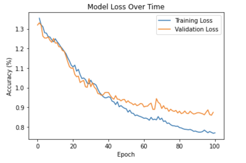
Validation and Training Accuracy Over Time
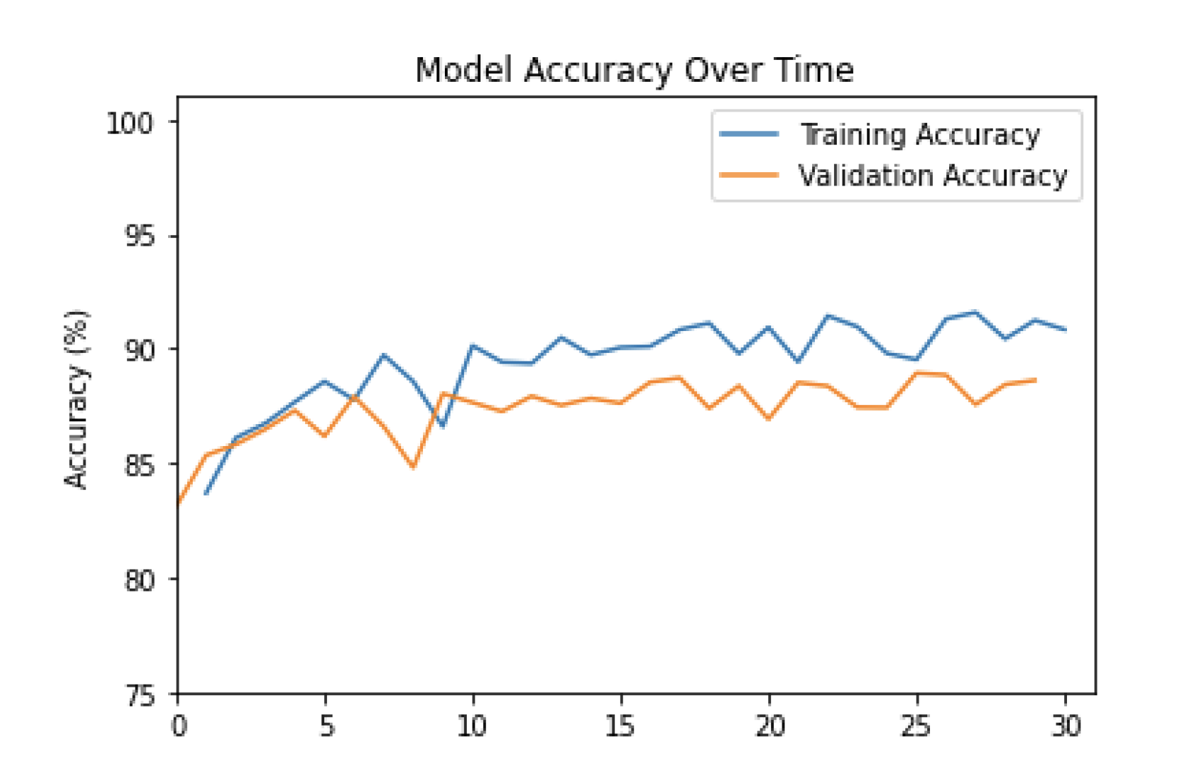
We see the accuracy increasing over time. It began fairly high with the first iteration around 82%, and it increased to around 90% for training and 87% for validation. Adding more layers, larger kernels, and trying other forms of nonlinear units may improve this accuracy
Per Class Accuracy
| Clothing |
Accuracy |
| T-shirt/top |
85 % |
|
Trouser
|
96 %
|
|
Pullover
|
83 %
|
|
Dress
|
90 %
|
|
Coat
|
68 %
|
|
Sandal
|
97 %
|
|
Shirt
|
71 %
|
|
Sneaker
|
95 %
|
|
Bag
|
96 %
|
|
Ankle Boot
|
95 %
|
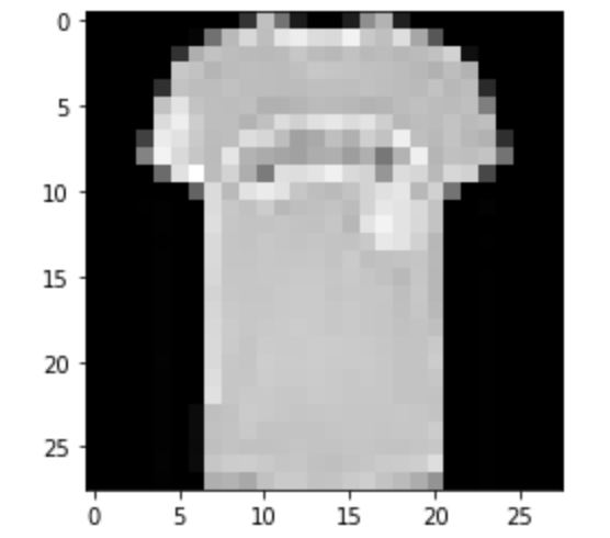
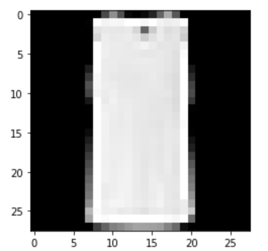
These are all fairly high accuracies, with many being above 90%. Looking at the sample results below, I noticed that even I am having difficulty determining some of those images, so the inherent quality of the dataset may be preventing higher accuracy results.
Sample Results
|
T-Shirt/Top: Correct
|
Correct
|
Predicted: Shirt
|
Predicted: Pullover
|
|
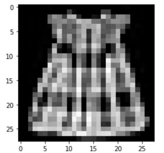
Trousers: Correct
|
Correct
|
Predicted: Dress
|
Predicted: Dress
|
|
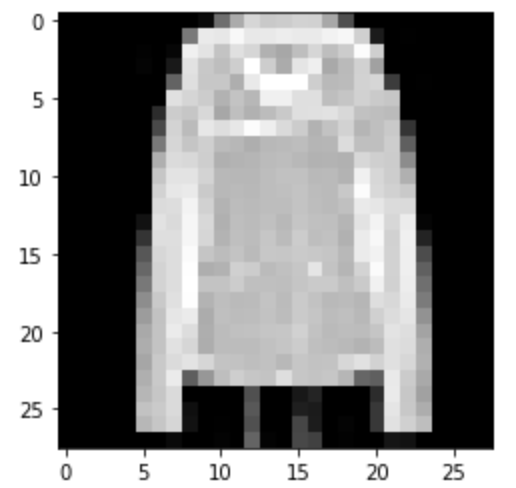
Pullover: Correct
|
Correct
|
Predicted: Shirt
|
Predicted: Coat
|
|
Dress: Correct
|
Correct
|
Predicted: Shirt
|
Predicted: Shirt
|
|
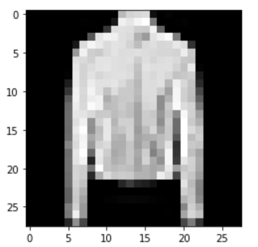
Coat: Correct
|
Correct
|
Predicted: Shirt
|
Predicted: Pullover
|
|
Sandal: Correct
|
Correct
|
Predicted: Sneaker
|
Predicted: Sneaker
|
|
Shirt: Correct
|
Correct
|
Predicted: T-shirt/Top
|
Predicted: T-shirt/Top
|
|
Sneaker: Correct
|
Correct
|
Predicted: Ankle Boot
|
Predicted: Sandal
|
|
Bag: Correct
|
Correct
|
Predicted: Trouser
|
Predicted: Dress
|
|
Ankle Boot: Correct
|
Correct
|
Predicted: Sneaker
|
Predicted: Sneaker
|
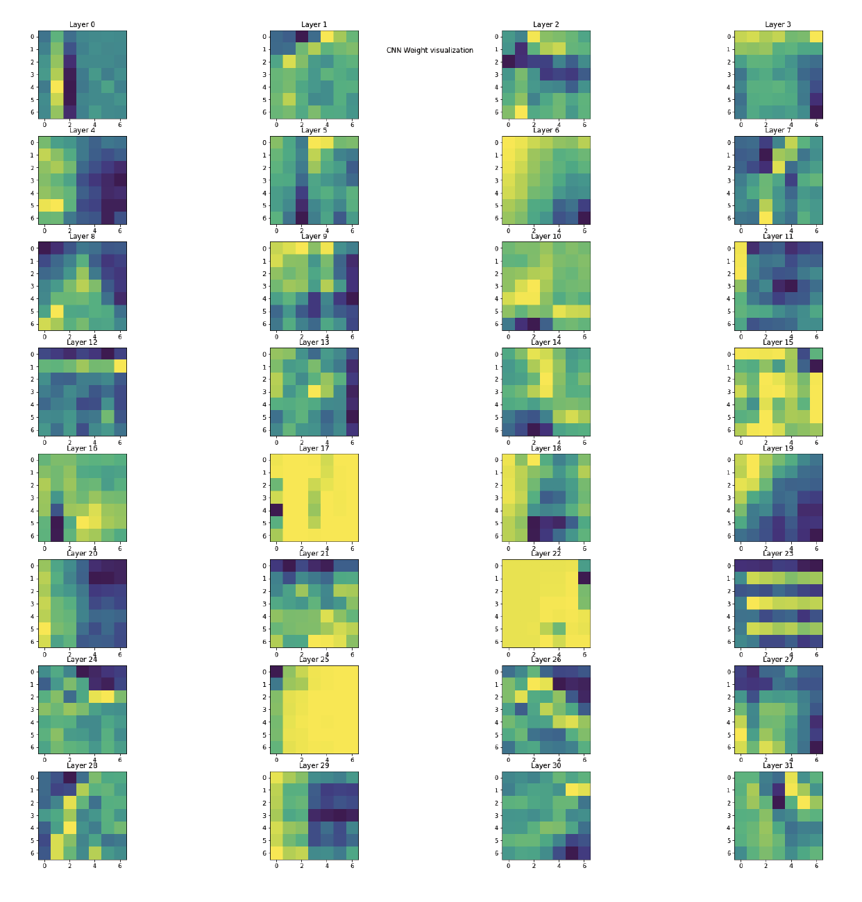
Filter Visualization
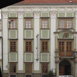
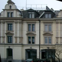
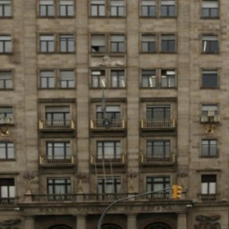
Semantic Segmentation
Using the Mini Facade dataset, I trained an NN to segment the images into their various components.
Network Structure
This network has a six layer convolution/max pooling setup, with the following parameters below, designed to maintain the 256 x 256 image dimensions:
| Layer Parameters |
|
| Kernels |
7 |
| Padding |
3 |
| Stride |
1 |
| Start Channel |
3 |
| Internal Channels |
20 |
| Final Channel |
Number of Classes |
|
|
|
| Global Parameters |
|
| Criterion |
Cross-Entropy Loss |
| Optimizer |
Adam |
| Learning Rate |
0.0005 |
| Weight Decay |
0.01 |
| Nonlinearity |
ELU |
Tuning of the Network
I started by establishing the 6 layers and determining the kernel sizes, padding, and channels needed to maintain proper input output dimensions. For simplicity, I made the padding, kernel sizes, and internal channels constant. With an odd kernel size and padding = (kernel size - 1) / 2, each layer maintained the input dimensions. Having an initial channel of 3 for RGB and output of number of classes solidified this structure as proper dimensions. I then tuned the learning rate to as high as possible while avoiding oscillations in convergence, and then increased the kernel size and internal channel number until I didn't notice a change anymore. I tuned the weight decay to offset the training bias without losing too much of the training data information. I still had fairly low average precision, but when I replaced the ReLU nonlinearities with ELU linearities my average precision reached the 45 % goal. I then trained on the entire training dataset and achieved the results below.
Results
Validation and Training Loss Over Time
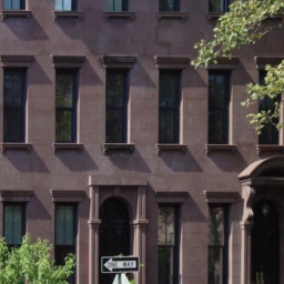
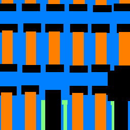
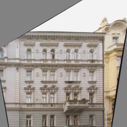
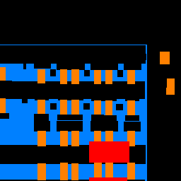
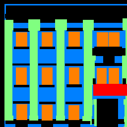
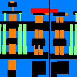
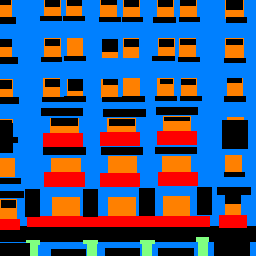
Sample Images
| Input |
Ground Truth |
Output |
|

|
|
|
|

|
|

|
|
|
|

|
|
|

|
Average Precision Values
| Class |
Color |
Average Precision |
| Others |
Black |
0.6140 |
| Facade |
Blue |
0.7309 |
| Pillar |
Green |
0.1175 |
| Window |
Orange |
0.7696 |
| Balcony |
Red |
0.3960 |
|
|
|
Total Average Precision:
|
0.5256
|
While we see very low average precistion with pillar segmentation, facades, windows, and others are segmented decently well, helping us achieve an average precision of 0.5256